`vegas` Module¶

Introduction¶

The key Python objects and functions supported by the vegas module are:

vegas.Integrator — an object describing a multidimensional integration operator. Such objects contain information about the integration volume, and also about optimal remappings of the integration variables based upon the last integral evaluated using the object.

vegas.AdaptiveMap — an object describing the remappings used by vegas.

vegas.RAvg — an object describing the result of a vegas integration. vegas returns the weighted average of the integral estimates from each vegas iteration as an object of class vegas.RAvg. These are Gaussian random variables — that is, they have a mean and a standard deviation — but also contain information about the iterations vegas used in generating the result.

vegas.RAvgArray — an array version of vegas.RAvg used when the integrand is array-valued.

vegas.RAvgDict — a dictionary version of vegas.RAvg used when the integrand is dictionary-valued.

vegas.lbatchintegrand() — a decorator that labels a function as an lbatch integrand.

vegas.rbatchintegrand() — a decorator that labels a function as an rbatch integrand.

vegas.PDFIntegrator — a specialized integrator for evaluating expectation values with arbitrary probability density functions.

vegas.PDFEV — an expectation value from vegas.PDFIntegrator.

vegas.PDFEVArray — an array of expectation values from vegas.PDFIntegrator.

vegas.PDFEVDict — a dictionary of expectation values from vegas.PDFIntegrator.

These are described in detail below.

Integrator Objects¶

The central component of the vegas package is the integrator class:

class vegas.Integrator¶

Adaptive multidimensional Monte Carlo integration.

vegas.Integrator objects make Monte Carlo estimates of multidimensional functions f(x) where x[d] is a point in the integration volume:

integ = vegas.Integrator(integration_region)

result = integ(f, nitn=10, neval=10000)

The integator makes nitn estimates of the integral, each using at most neval samples of the integrand, as it adapts to the specific features of the integrand. Successive estimates (iterations) typically improve in accuracy until the integrator has fully adapted. The integrator returns the weighted average of all nitn estimates, together with an estimate of the statistical (Monte Carlo) uncertainty in that estimate of the integral. The result is an object of type RAvg (which is derived from gvar.GVar).

Integrands f(x) return numbers, arrays of numbers (any shape), or dictionaries whose values are numbers or arrays (any shape). Each number returned by an integrand corresponds to a different integrand. When arrays are returned, vegas adapts to the first number in the flattened array. When dictionaries are returned, vegas adapts to the first number in the value corresponding to the first key.

vegas can generate integration points in batches for integrands built from classes derived from vegas.LBatchIntegrand, or integrand functions decorated by vegas.lbatchintegrand(). Batch integrands are typically much faster, especially if they are coded in Cython or C/C++ or Fortran.

vegas.Integrators have a large number of parameters but the only ones that most people will care about are: the number nitn of iterations of the vegas algorithm; the maximum number neval of integrand evaluations per iteration; and the damping parameter alpha, which is used to slow down the adaptive algorithms when they would otherwise be unstable (e.g., with very peaky integrands). Setting parameter analyzer=vegas.reporter() is sometimes useful, as well, since it causes vegas to print (on sys.stdout) intermediate results from each iteration, as they are produced. This helps when each iteration takes a long time to complete (e.g., longer than an hour) because it allows you to monitor progress as it is being made (or not).

Parameters:

map (array, dictionary, vegas.AdaptiveMap or vegas.Integrator) –
The integration region is specified by an array map[d, i] where d is the direction and i=0,1 specify the lower and upper limits of integration in direction d. Integration points x are packaged as arrays x[d] when passed to the integrand f(x).

More generally, the integrator packages integration points in multidimensional arrays x[d1, d2..dn] when the integration limits are specified by map[d1, d2...dn, i] with i=0,1. These arrays can have any shape.

Alternatively, the integration region can be specified by a dictionary whose values map[key] are either 2-tuples or arrays of 2-tuples corresponding to the lower and upper integration limits for the corresponding variables. Then integration points xd are packaged as dictionaries having the same structure as map but with the integration limits replaced by the values of the variables: for example,
```
map = dict(r=(0, 1), phi=[(0, np.pi), (0, 2 * np.pi)])
```
indicates a three-dimensional integral over variables r (from 0 to 1), phi[0] (from 0 to np.pi), and phi[1] (from 0 to 2*np.pi). In this case integrands f(xd) have dictionary arguments xd where xd['r'], xd['phi'][0], and xd['phi'][1] correspond to the integration variables.

Finally map could be the integration map from another vegas.Integrator, or that vegas.Integrator itself. In this case the grid is copied from the existing integrator.
uses_jac (bool) – Setting uses_jac=True causes vegas to call the integrand with two arguments: fcn(x, jac=jac). The second argument is the Jacobian jac[d] = dx[d]/dy[d] of the vegas map. The integral over x[d] of 1/jac[d] equals 1 (exactly). The default setting is uses_jac=False.
nitn (positive int) – The maximum number of iterations used to adapt to the integrand and estimate its value. The default value is 10; typical values range from 10 to 20.
neval (positive int) – Approximate number of integrand evaluations in each iteration of the vegas algorithm. Increasing neval increases the precision: statistical errors should fall at least as fast as sqrt(1./neval) and often fall much faster. The default value is 1000; real problems often require 10–10,000 times more evaluations than this.
nstrat (int array) – nstrat[d] specifies the number of stratifications to use in direction d. By default this parameter is set automatically, based on parameter neval, with nstrat[d] approximately the same for every d. Specifying nstrat explicitly makes it possible to concentrate stratifications in directions where they are most needed. If nstrat is set but neval is not, neval is set equal to 2*prod(nstrat)/(1-neval_frac).
alpha (float) – Damping parameter controlling the remapping of the integration variables as vegas adapts to the integrand. Smaller values slow adaptation, which may be desirable for difficult integrands. Small or zero alphas are also sometimes useful after the grid has adapted, to minimize fluctuations away from the optimal grid. The default value is 0.5.
beta (float) – Damping parameter controlling the redistribution of integrand evaluations across hypercubes in the stratified sampling of the integral (over transformed variables). Smaller values limit the amount of redistribution. The theoretically optimal value is 1; setting beta=0 prevents any redistribution of evaluations. The default value is 0.75.
neval_frac (float) – Approximate fraction of function evaluations used for adaptive stratified sampling. vegas distributes (1-neval_frac)*neval integrand evaluations uniformly over all hypercubes, with at least 2 evaluations per hypercube. The remaining neval_frac*neval evaluations are concentrated in hypercubes where the errors are largest. Increasing neval_frac makes more integrand evaluations available for adaptive stratified sampling, but reduces the number of hypercubes, which limits the algorithm’s ability to adapt. Ignored when beta=0. Default is neval_frac=0.75.
adapt (bool) – Setting adapt=False prevents further adaptation by vegas. Typically this would be done after training the vegas.Integrator on an integrand, in order to stabilize further estimates of the integral. vegas uses unweighted averages to combine results from different iterations when adapt=False. The default setting is adapt=True.
nproc (int or None) –
Number of processes/processors used to evalute the integrand. If nproc>1 Python’s multiprocessing module is used to spread integration points across multiple processors, thereby potentially reducing the time required to evaluate the integral. There is a significant overhead involved in using multiple processors so this option is useful only when the integrand is expensive to evaluate. When using the multiprocessing module in its default mode for MacOS and Windows, it is important that the main module can be safely imported (i.e., without launching new processes). This can be accomplished with some version of the if __name__ == '__main__`: construct in the main module: e.g.,
```
if __name__ == '__main__':
    main()
```
This is not an issue on other Unix platforms. See the multiprocessing documentation for more information. Note that setting nproc greater than 1 disables MPI support. Set nproc=None to use all the processors on the machine (equivalent to nproc=os.cpu_count()). Default value is nproc=1. (Requires Python 3.3 or later.)

Note that nproc has nothing to do with MPI support. The number of MPI processors is specified outside Python (via, for example, mpirun -np 8 python script.py on the command line).
analyzer –
An object with methods

analyzer.begin(itn, integrator)

analyzer.end(itn_result, result)

where: begin(itn, integrator) is called at the start of each vegas iteration with itn equal to the iteration number and integrator equal to the integrator itself; and end(itn_result, result) is called at the end of each iteration with itn_result equal to the result for that iteration and result equal to the cummulative result of all iterations so far. Setting analyzer=vegas.reporter(), for example, causes vegas to print out a running report of its results as they are produced. The default is analyzer=None.
min_neval_batch (positive int) – The minimum number of integration points to be passed together to the integrand when using vegas in batch mode. The default value is 50,000. Larger values may be lead to faster evaluations, but at the cost of more memory for internal work arrays. The last batch is usually smaller than this limit, as it is limited by neval.
max_neval_hcube (positive int) – Maximum number of integrand evaluations per hypercube in the stratification. The default value is 50,000. Larger values might allow for more adaptation (when beta>0), but also allow for more over-shoot when adapting to sharp peaks. Larger values also can result in large internal work arrasy.
minimize_mem (bool) – When True, vegas minimizes internal workspace by moving some of its data to a disk file. This increases execution time (slightly) and results in temporary files, but might be desirable when the number of evaluations is very large (e.g., neval=1e9). minimize_mem=True requires the h5py Python module.
max_mem (positive float) – Maximum number of floats allowed in internal work arrays (approx.). A MemoryError is raised if the work arrays are too large, in which case one might want to reduce min_neval_batch or max_neval_hcube, or set minimize_mem=True (or increase max_mem if there is enough RAM). Default value is 1e9.
maxinc_axis (positive int) – The maximum number of increments per axis allowed for the x-space grid. The default value is 1000; there is probably little need to use other values.
rtol (float) – Relative error in the integral estimate at which point the integrator can stop. The default value is 0.0 which turns off this stopping condition. This stopping condition can be quite unreliable in early iterations, before vegas has converged. Use with caution, if at all.
atol (float) – Absolute error in the integral estimate at which point the integrator can stop. The default value is 0.0 which turns off this stopping condition. This stopping condition can be quite unreliable in early iterations, before vegas has converged. Use with caution, if at all.
ran_array_generator – Replacement function for the default random number generator. ran_array_generator(size) should create random numbers uniformly distributed between 0 and 1 in an array whose dimensions are specified by the integer-valued tuple size. Setting ran_array_generator to None restores the default generator (from gvar).
sync_ran (bool) – If True (default), the default random number generator is synchronized across all processors when using MPI. If False, vegas does no synchronization (but the random numbers should synchronized some other way). Ignored if not using MPI.
adapt_to_errors (bool) –
adapt_to_errors=False causes vegas to remap the integration variables to emphasize regions where |f(x)| is largest. This is the default mode.

adapt_to_errors=True causes vegas to remap variables to emphasize regions where the Monte Carlo error is largest. This might be superior when the number of the number of stratifications (self.nstrat) in the y grid is large (> 100). It is typically useful only in one or two dimensions.
uniform_nstrat (bool) – If True, requires that the nstrat[d] be equal for all d. If False (default), the algorithm maximizes the number of stratifications while requiring |nstrat[d1] - nstrat[d2]| <= 1. This parameter is ignored if nstrat is specified explicitly.
mpi – Setting mpi=False (default) disables mpi support in vegas even if mpi is available; setting mpi=True allows use of mpi provided module mpi4py is installed.

Methods:

__call__(fcn, save=None, saveall=None, **kargs)¶

Integrate integrand fcn.

A typical integrand has the form, for example:

def f(x):
    return x[0] ** 2 + x[1] ** 4

The argument x[d] is an integration point, where index d=0... represents direction within the integration volume.

Integrands can be array-valued, representing multiple integrands: e.g.,

def f(x):
    return [x[0] ** 2, x[0] / x[1]]

The return arrays can have any shape. Dictionary-valued integrands are also supported: e.g.,

def f(x):
    return dict(a=x[0] ** 2, b=[x[0] / x[1], x[1] / x[0]])

Integrand functions that return arrays or dictionaries are useful for multiple integrands that are closely related, and can lead to substantial reductions in the errors for ratios or differences of the results.

Integrand’s take dictionaries as arguments when Integrator keyword map is set equal to a dictionary. For example, with

map = dict(r=(0,1), theta=(0, np.pi), phi=(0, 2*np.pi))

the volume of a unit sphere is obtained by integrating

def f(xd):
    r = xd['r']
    theta = xd['theta']
    return r ** 2 * np.sin(theta)

It is usually much faster to use vegas in batch mode, where integration points are presented to the integrand in batches. A simple batch integrand might be, for example:

@vegas.lbatchintegrand
def f(x):
    return x[:, 0] ** 2 + x[:, 1] ** 4

where decorator @vegas.lbatchintegrand tells vegas that the integrand processes integration points in batches. The array x[i, d] represents a collection of different integration points labeled by i=0.... (The number of points is controlled vegas.Integrator parameter min_neval_batch.)

Batch mode is particularly useful (and fast) when the integrand is coded in Cython. Then loops over the integration points can be coded explicitly, avoiding the need to use numpy’s whole-array operators if they are not well suited to the integrand.

The batch index is always first (leftmost) for lbatch integrands, as above. It is also possible to create batch integrands where the batch index is the last (rightmost) index: for example,

@vegas.rbatchintegrand
def f(x):
    return x[0, :] ** 2 + x[1, :] ** 4

Batch integrands can also be constructed from classes derived from vegas.LBatchIntegrand or vegas.RBatchIntegrand.

Any vegas parameter can also be reset: e.g., self(fcn, nitn=20, neval=1e6).

Parameters:

fcn (callable) – Integrand function.
save (str or file or None) –
Writes results into pickle file specified by save at the end of each iteration. For example, setting save='results.pkl' means that the results returned by the last vegas iteration can be reconstructed later using:
```
import pickle
with open('results.pkl', 'rb') as ifile:
    results = pickle.load(ifile)
```
Ignored if save=None (default).
saveall (str or file or None) –
Writes (results, integrator) into pickle file specified by saveall at the end of each iteration. For example, setting saveall='allresults.pkl' means that the results returned by the last vegas iteration, together with a clone of the (adapted) integrator, can be reconstructed later using:
```
import pickle
with open('allresults.pkl', 'rb') as ifile:
    results, integrator = pickle.load(ifile)
```
Ignored if saveall=None (default).

Returns:

Monte Carlo estimate of the integral of fcn(x) as an object of type vegas.RAvg, vegas.RAvgArray, or vegas.RAvgDict.

set(ka={}, **kargs)¶

Reset default parameters in integrator.

Usage is analogous to the constructor for vegas.Integrator: for example,

old_defaults = integ.set(neval=1e6, nitn=20)

resets the default values for neval and nitn in vegas.Integrator integ. A dictionary, here old_defaults, is returned. It can be used to restore the old defaults using, for example:

integ.set(old_defaults)

settings(ngrid=0)¶

Assemble summary of integrator settings into string.

Parameters:: ngrid (int) – Number of grid nodes in each direction to include in summary. The default is 0.
Returns:: String containing the settings.

random(yield_hcube=False, yield_y=False)¶

Low-level iterator over integration points and weights.

This method creates an iterator that returns integration points from vegas, and their corresponding weights in an integral. Each point x[d] is accompanied by the weight assigned to that point by vegas when estimating an integral. Optionally it will also return the index of the hypercube containing the integration point and/or the y-space coordinates:

integ.random()  yields  x, wgt

integ.random(yield_hcube=True) yields x, wgt, hcube

integ.random(yield_y=True) yields x, y, wgt

integ.random(yield_hcube=True, yield_y=True) yields x, y, wgt, hcube

The number of integration points returned by the iterator corresponds to a single iteration.

random_batch(yield_hcube=False, yield_y=False)¶

Low-level batch iterator over integration points and weights.

This method creates an iterator that returns integration points from vegas, and their corresponding weights in an integral. The points are provided in arrays x[i, d] where i=0... labels the integration points in a batch and d=0... labels direction. The corresponding weights assigned by vegas to each point are provided in an array wgt[i].

Optionally the integrator will also return the indices of the hypercubes containing the integration points and/or the y-space coordinates of those points:

integ.random_batch()  yields  x, wgt

integ.random_batch(yield_hcube=True) yields x, wgt, hcube

integ.random_batch(yield_y=True) yields x, y, wgt

integ.random_batch(yield_hcube=True, yield_y=True) yields x, y, wgt, hcube

The number of integration points returned by the iterator corresponds to a single iteration. The number in a batch is controlled by parameter nhcube_batch.

AdaptiveMap Objects¶

vegas’s remapping of the integration variables is handled by a vegas.AdaptiveMap object, which maps the original integration variables x into new variables y in a unit hypercube. Each direction has its own map specified by a grid in x space:

$x_0 &= a \\ x_1 &= x_0 + \Delta x_0 \\ x_2 &= x_1 + \Delta x_1 \\ \cdots \\ x_N &= x_{N-1} + \Delta x_{N-1} = b$

where $a$ and $b$ are the limits of integration. The grid specifies the transformation function at the points $y=i/N$ for $i=0,1\ldots N$ :

$x(y\!=\!i/N) = x_i$

Linear interpolation is used between those points. The Jacobian for this transformation is:

$J(y) = J_i = N \Delta x_i$

vegas adjusts the increments sizes to optimize its Monte Carlo estimates of the integral. This involves training the grid. To illustrate how this is done with vegas.AdaptiveMaps consider a simple two dimensional integral over a unit hypercube with integrand:

def f(x):
   return x[0] * x[1] ** 2

We want to create a grid that optimizes uniform Monte Carlo estimates of the integral in y space. We do this by sampling the integrand at a large number ny of random points y[j, d], where j=0...ny-1 and d=0,1, uniformly distributed throughout the integration volume in y space. These samples be used to train the grid using the following code:

import vegas
import numpy as np

def f(x):
   return x[0] * x[1] ** 2

m = vegas.AdaptiveMap([[0, 1], [0, 1]], ninc=5)

ny = 1000
y = np.random.uniform(0., 1., (ny, 2))  # 1000 random y's

x = np.empty(y.shape, float)            # work space
jac = np.empty(y.shape[0], float)
f2 = np.empty(y.shape[0], float)

print('intial grid:')
print(m.settings())

for itn in range(5):                    # 5 iterations to adapt
   m.map(y, x, jac)                     # compute x's and jac

   for j in range(ny):                  # compute training data
      f2[j] = (jac[j] * f(x[j])) ** 2

   m.add_training_data(y, f2)           # adapt
   m.adapt(alpha=1.5)

   print('iteration %d:' % itn)
   print(m.settings())

In each of the 5 iterations, the vegas.AdaptiveMap adjusts the map, making increments smaller where f2 is larger and larger where f2 is smaller. The map converges after only 2 or 3 iterations, as is clear from the output:

initial grid:
    grid[ 0] = [ 0.   0.2  0.4  0.6  0.8  1. ]
    grid[ 1] = [ 0.   0.2  0.4  0.6  0.8  1. ]

iteration 0:
    grid[ 0] = [ 0.     0.412  0.62   0.76   0.883  1.   ]
    grid[ 1] = [ 0.     0.506  0.691  0.821  0.91   1.   ]

iteration 1:
    grid[ 0] = [ 0.     0.428  0.63   0.772  0.893  1.   ]
    grid[ 1] = [ 0.     0.531  0.713  0.832  0.921  1.   ]

iteration 2:
    grid[ 0] = [ 0.     0.433  0.63   0.772  0.894  1.   ]
    grid[ 1] = [ 0.     0.533  0.714  0.831  0.922  1.   ]

iteration 3:
    grid[ 0] = [ 0.     0.435  0.631  0.772  0.894  1.   ]
    grid[ 1] = [ 0.     0.533  0.715  0.831  0.923  1.   ]

iteration 4:
    grid[ 0] = [ 0.     0.436  0.631  0.772  0.895  1.   ]
    grid[ 1] = [ 0.     0.533  0.715  0.831  0.924  1.   ]

The grid increments along direction 0 shrink at larger values x[0], varying as 1/x[0]. Along direction 1 the increments shrink more quickly varying like 1/x[1]**2.

vegas samples the integrand in order to estimate the integral. It uses those same samples to train its vegas.AdaptiveMap in this fashion, for use in subsequent iterations of the algorithm.

class vegas.AdaptiveMap¶

Adaptive map y->x(y) for multidimensional y and x.

An AdaptiveMap defines a multidimensional map y -> x(y) from the unit hypercube, with 0 <= y[d] <= 1, to an arbitrary hypercube in x space. Each direction is mapped independently with a Jacobian that is tunable (i.e., “adaptive”).

The map is specified by a grid in x-space that, by definition, maps into a uniformly spaced grid in y-space. The nodes of the grid are specified by grid[d, i] where d is the direction (d=0,1...dim-1) and i labels the grid point (i=0,1...N). The mapping for a specific point y into x space is:

y[d] -> x[d] = grid[d, i(y[d])] + inc[d, i(y[d])] * delta(y[d])

where i(y)=floor(y*N), delta(y)=y*N - i(y), and inc[d, i] = grid[d, i+1] - grid[d, i]. The Jacobian for this map,

dx[d]/dy[d] = inc[d, i(y[d])] * N,

is piece-wise constant and proportional to the x-space grid spacing. Each increment in the x-space grid maps into an increment of size 1/N in the corresponding y space. So regions in x space where inc[d, i] is small are stretched out in y space, while larger increments are compressed.

The x grid for an AdaptiveMap can be specified explicitly when the map is created: for example,

m = AdaptiveMap([[0, 0.1, 1], [-1, 0, 1]])

creates a two-dimensional map where the x[0] interval (0,0.1) and (0.1,1) map into the y[0] intervals (0,0.5) and (0.5,1) respectively, while x[1] intervals (-1,0) and (0,1) map into y[1] intervals (0,0.5) and (0.5,1).

More typically, an uniform map with ninc increments is first created: for example,

m = AdaptiveMap([[0, 1], [-1, 1]], ninc=1000)

creates a two-dimensional grid, with 1000 increments in each direction, that spans the volume 0<=x[0]<=1, -1<=x[1]<=1. This map is then trained with data f[j] corresponding to ny points y[j, d], with j=0...ny-1, (usually) uniformly distributed in y space: for example,

m.add_training_data(y, f)
m.adapt(alpha=1.5)

m.adapt(alpha=1.5) shrinks grid increments where f[j] is large, and expands them where f[j] is small. Usually one has to iterate over several sets of ys and fs before the grid has fully adapted.

The speed with which the grid adapts is determined by parameter alpha. Large (positive) values imply rapid adaptation, while small values (much less than one) imply slow adaptation. As in any iterative process that involves random numbers, it is usually a good idea to slow adaptation down in order to avoid instabilities caused by random fluctuations.

Parameters:

grid (list of arrays) – Initial x grid, where grid[d][i] is the i-th node in direction d. Different directions can have different numbers of nodes.
ninc (int or array or None) – ninc[d] (or ninc, if it is a number) is the number of increments along direction d in the new x grid. The new grid is designed to give the same Jacobian dx(y)/dy as the original grid. The default value, ninc=None, leaves the grid unchanged.

Attributes and methods:

dim¶: Number of dimensions.

ninc¶: ninc[d] is the number increments in direction d.

grid¶: The nodes of the grid defining the maps are self.grid[d, i] where d=0... specifies the direction and i=0...self.ninc the node.

inc¶

The increment widths of the grid:

self.inc[d, i] = self.grid[d, i + 1] - self.grid[d, i]

adapt(alpha=0.0, ninc=None)¶

Adapt grid to accumulated training data.

self.adapt(...) projects the training data onto each axis independently and maps it into x space. It shrinks x-grid increments in regions where the projected training data is large, and grows increments where the projected data is small. The grid along any direction is unchanged if the training data is constant along that direction.

The number of increments along a direction can be changed by setting parameter ninc (array or number).

The grid does not change if no training data has been accumulated, unless ninc is specified, in which case the number of increments is adjusted while preserving the relative density of increments at different values of x.

Parameters:

alpha (double) – Determines the speed with which the grid adapts to training data. Large (postive) values imply rapid evolution; small values (much less than one) imply slow evolution. Typical values are of order one. Choosing alpha<0 causes adaptation to the unmodified training data (usually not a good idea).
ninc (int or array or None) – The number of increments in the new grid is ninc[d] (or ninc, if it is a number) in direction d. The number is unchanged from the old grid if ninc is omitted (or equals None, which is the default).

add_training_data(y, f, ny=-1)¶

Add training data f for y-space points y.

Accumulates training data for later use by self.adapt(). Grid increments will be made smaller in regions where f is larger than average, and larger where f is smaller than average. The grid is unchanged (converged?) when f is constant across the grid.

Parameters:

y (array) – y values corresponding to the training data. y is a contiguous 2-d array, where y[j, d] is for points along direction d.
f (array) – Training function values. f[j] corresponds to point y[j, d] in y-space.
ny (int) – Number of y points: y[j, d] for d=0...dim-1 and j=0...ny-1. ny is set to y.shape[0] if it is omitted (or negative).

adapt_to_samples(x, f, nitn=5, alpha=1.0, nproc=1)¶

Adapt map to data {x, f(x)}.

Replace grid with one that is optimized for integrating function f(x). New grid is found iteratively

Parameters:

x (array) – x[:, d] are the components of the sample points in direction d=0,1...self.dim-1.
f (callable or array) – Function f(x) to be adapted to. If f is an array, it is assumes to contain values f[i] corresponding to the function evaluated at points x[i].
nitn (int) – Number of iterations to use in adaptation. Default is nitn=5.
alpha (float) – Damping parameter for adaptation. Default is alpha=1.0. Smaller values slow the iterative adaptation, to improve stability of convergence.
nproc (int or None) –
Number of processes/processors to use. If nproc>1 Python’s multiprocessing module is used to spread the calculation across multiple processors. There is a significant overhead involved in using multiple processors so this option is useful mainly when very high dimenions or large numbers of samples are involved. When using the multiprocessing module in its default mode for MacOS and Windows, it is important that the main module can be safely imported (i.e., without launching new processes). This can be accomplished with some version of the if __name__ == '__main__`: construct in the main module: e.g.,
```
if __name__ == '__main__':
    main()
```
This is not an issue on other Unix platforms. See the multiprocessing documentation for more information. Set nproc=None to use all the processors on the machine (equivalent to nproc=os.cpu_count()). Default value is nproc=1. (Requires Python 3.3 or later.)

__call__(y)¶

Return x values corresponding to y.

y can be a single dim-dimensional point, or it can be an array y[i,j, ..., d] of such points (d=0..dim-1).

If y=None (default), y is set equal to a (uniform) random point in the volume.

jac(y)¶

Return the map’s Jacobian at y.

y can be a single dim-dimensional point, or it can be an array y[i,j,...,d] of such points (d=0..dim-1). Returns an array jac where jac[i,j,...] is the (multidimensional) Jacobian (dx/dy) corresponding to y[i,j,...].

jac1d(y)¶

Return the map’s Jacobian at y for each direction.

y can be a single dim-dimensional point, or it can be an array y[i,j,...,d] of such points (d=0..dim-1). Returns an array jac where jac[i,j,...,d] is the (one-dimensional) Jacobian (dx[d]/dy[d]) corresponding to y[i,j,...,d].

make_uniform(ninc=None)¶

Replace the grid with a uniform grid.

The new grid has ninc[d] (or ninc, if it is a number) increments along each direction if ninc is specified. If ninc=None (default), the new grid has the same number of increments in each direction as the old grid.

map(y, x, jac, ny=-1)¶

Map y to x, where jac is the Jacobian (dx/dy).

y[j, d] is an array of ny y-values for direction d. x[j, d] is filled with the corresponding x values, and jac[j] is filled with the corresponding Jacobian values. x and jac must be preallocated: for example,

x = numpy.empty(y.shape, float)
jac = numpy.empty(y.shape[0], float)

Parameters:

y (array) – y values to be mapped. y is a contiguous 2-d array, where y[j, d] contains values for points along direction d.
x (array) – Container for x[j, d] values corresponding to y[j, d]. Must be a contiguous 2-d array.
jac (array) – Container for Jacobian values jac[j] (= dx/dy) corresponding to y[j, d]. Must be a contiguous 1-d array.
ny (int) – Number of y points: y[j, d] for d=0...dim-1 and j=0...ny-1. ny is set to y.shape[0] if it is omitted (or negative).

invmap(x, y, jac, nx=-1)¶

Map x to y, where jac is the Jacobian (dx/dy).

y[j, d] is an array of ny y-values for direction d. x[j, d] is filled with the corresponding x values, and jac[j] is filled with the corresponding Jacobian values. x and jac must be preallocated: for example,

x = numpy.empty(y.shape, float)
jac = numpy.empty(y.shape[0], float)

Parameters:

x (array) – x values to be mapped to y-space. x is a contiguous 2-d array, where x[j, d] contains values for points along direction d.
y (array) – Container for y[j, d] values corresponding to x[j, d]. Must be a contiguous 2-d array
jac (array) – Container for Jacobian values jac[j] (= dx/dy) corresponding to y[j, d]. Must be a contiguous 1-d array
nx (int) – Number of x points: x[j, d] for d=0...dim-1 and j=0...nx-1. nx is set to x.shape[0] if it is omitted (or negative).

show_grid(ngrid=40, shrink=False)¶

Display plots showing the current grid.

Parameters:

ngrid (int) – The number of grid nodes in each direction to include in the plot. The default is 40.
axes – List of pairs of directions to use in different views of the grid. Using None in place of a direction plots the grid for only one direction. Omitting axes causes a default set of pairings to be used.
shrink – Display entire range of each axis if False; otherwise shrink range to include just the nodes being displayed. The default is False.
plotter – matplotlib plotter to use for plots; plots are not displayed if set. Ignored if None, and plots are displayed using matplotlib.pyplot.

settings(ngrid=5)¶

Create string with information about grid nodes.

Creates a string containing the locations of the nodes in the map grid for each direction. Parameter ngrid specifies the maximum number of nodes to print (spread evenly over the grid).

extract_grid()¶: Return a list of lists specifying the map’s grid.

clear()¶: Clear information accumulated by AdaptiveMap.add_training_data().

PDFIntegrator Objects¶

Expectation values using probability density functions defined by collections of Gaussian random variables (see gvar) can be evaluated using the following specialized integrator:

class vegas.PDFIntegrator(g, limit=1e15, scale=1., svdcut=1e-15)¶

vegas integrator for PDF expectation values.

PDFIntegrator(param, pdf) creates a vegas integrator that evaluates expectation values of arbitrary functions f(p) with respect to the probability density function pdf(p), where p is a point in the parameter space defined by param.

param is a collection of gvar.GVars (Gaussian random variables) that together define a multi-dimensional Gaussian distribution with the same parameter space as the distribution described by pdf(p). PDFIntegrator internally re-expresses the integrals over these parameters in terms of new variables that emphasize the region defined by param (i.e., the region where the PDF associated with the param’s Gaussian distribution is large). The new variables are also aligned with the principal axes of param’s correlation matrix, to facilitate integration.

param’s means and covariances are chosen to emphasize the important regions of the pdf’s distribution (e.g., param might be set equal to the prior in a Bayesian analysis). param is used to define and optimize the integration variables; it does not affect the values of the integrals but can have a big effect on the accuracy.

The Gaussian PDF associated with param is used if pdf is unspecified (i.e., pdf=None, which is the default).

Typical usage is illustrated by the following code, where dictionary g specifies both the parameterization (param) and the PDF:

import vegas
import gvar as gv
import numpy as np

g = gv.BufferDict()
g['a'] = gv.gvar([10., 2.], [[1, 1.4], [1.4, 2]])
g['fb(b)'] = gv.BufferDict.uniform('fb', 2.9, 3.1)

g_ev = vegas.PDFIntegrator(g)

def f(p):
    a = p['a']
    b = p['b']
    return a[0] + np.fabs(a[1]) ** b

result = g_ev(f, neval=10_000, nitn=5)
print('<f(p)> =', result)

Here g indicates a three-dimensional distribution where the first two variables g['a'][0] and g['a'][1] are Gaussian with means 10 and 2, respectively, and covariance matrix [[1, 1.4], [1.4, 2.]]. The last variable g['b'] is uniformly distributed on interval [2.9, 3.1]. The result is: <f(p)> = 30.145(83).

PDFIntegrator evaluates integrals of both f(p) * pdf(p) and pdf(p). The expectation value of f(p) is the ratio of these two integrals (so pdf(p) need not be normalized). The result of a PDFIntegrator integration has an extra attribute, result.pdfnorm, which is the vegas estimate of the integral over the PDF.

Parameters:

param – A gvar.GVar, array of gvar.GVars, or dictionary, whose values are gvar.GVars or arrays of gvar.GVars, that specifies the integration parameters. When parameter pdf=None, the PDF is set equal to the Gaussian distribution corresponding to param.
pdf – The probability density function pdf(p). The PDF’s parameters p have the same layout as param (arrays or dictionary), with the same keys and/or shapes. The Gaussian PDF associated with param is used when pdf=None (default). Note that PDFs need not be normalized.
adapt_to_pdf (bool) – vegas adapts to the PDF when adapt_to_pdf=True (default). vegas adapts to pdf(p) * f(p) when calculating the expectation value of f(p) if adapt_to_pdf=False.
limit (positive float) – Integration variables are determined from param. limit limits the range of each variable to a region of size limit times the standard deviation on either side of the mean, where means and standard deviations are specified by param. This can be useful if the functions being integrated misbehave for large parameter values (e.g., numpy.exp overflows for a large range of arguments). Default is limit=100; results should become independent of limit as it is increased.
scale (positive float) – The integration variables are rescaled to emphasize parameter values of order scale times the standard deviation measured from the mean, where means and standard deviations are specified by param. The rescaling does not change the value of the integral but it can reduce uncertainties in the vegas estimate. Default is scale=1.0.
svdcut (non-negative float or None) – If not None, replace correlation matrix of param with a new matrix whose small eigenvalues are modified: eigenvalues smaller than svdcut times the maximum eigenvalue eig_max are replaced by svdcut*eig_max. This can ameliorate problems caused by roundoff errors when inverting the covariance matrix. It increases the uncertainty associated with the modified eigenvalues and so is conservative. Setting svdcut=None or svdcut=0 leaves the covariance matrix unchanged. Default is svdcut=1e-12.

All other keyword parameters are passed on to the the underlying vegas.Integrator; the uses_jac keyword is ignored.

Methods:

__call__(f=None, pdf=None, adapt_to_pdf=None, save=None, saveall=None, **kargs)¶

Estimate expectation value of function f(p).

Uses module vegas to estimate the integral of f(p) multiplied by the probability density function associated with g (i.e., pdf(p)). At the same time it integrates the PDF. The ratio of the two integrals is the expectation value.

Parameters:

f (function) – Function f(p) to integrate. Integral is the expectation value of the function with respect to the distribution. The function can return a number, an array of numbers, or a dictionary whose values are numbers or arrays of numbers. Setting f=None means that only the PDF is integrated. Integrals can be substantially faster if f(p) (and pdf(p) if set) are batch functions (see vegas documentation).
pdf – If specified, pdf(p) is used as the probability density function rather than the Gaussian PDF associated with g. The Gaussian PDF is used if pdf=None (default). Note that PDFs need not be normalized.
adapt_to_pdf (bool) – vegas adapts to the PDF when adapt_to_pdf=True (default). vegas adapts to pdf(p) * f(p) if adapt_to_pdf=False.
save (str or file or None) –
Writes results into pickle file specified by save at the end of each iteration. For example, setting save='results.pkl' means that the results returned by the last vegas iteration can be reconstructed later using:
```
import pickle
with open('results.pkl', 'rb') as ifile:
    results = pickle.load(ifile)
```
Ignored if save=None (default).
saveall (str or file or None) –
Writes (results, integrator) into pickle file specified by saveall at the end of each iteration. For example, setting saveall='allresults.pkl' means that the results returned by the last vegas iteration, together with a clone of the (adapted) integrator, can be reconstructed later using:
```
import pickle
with open('allresults.pkl', 'rb') as ifile:
    results, integrator = pickle.load(ifile)
```
Ignored if saveall=None (default).

All other keyword arguments are passed on to a vegas integrator; see the vegas documentation for further information.

Returns:: Expectation value(s) of f(p) as object of type vegas.PDFEV, vegas.PDFEVArray, or vegas.PDFEVDict.

stats(f, moments=False, histograms=False, **kargs)¶

Statistical analysis of function f(p).

Uses the vegas integrator to evaluate the expectation values and (co)variances of f(p) with respect to the probability density function associated with the PDFIntegrator. Typical usage is illustrated by:

>>> import gvar as gv
>>> import vegas
>>> g = gv.gvar(dict(a='1.0(5)', b='2(1)')) * gv.gvar('1.0(5)')
>>> g_ev = vegas.PDFIntegrator(g)
>>> g_ev(neval=10_000)    # adapt the integrator to the PDF
>>> @vegas.rbatchintegrand
... def f(p):
...     fp = dict(a=p['a'], b=p['b'])
...     fp['a**2 * b'] = p['a']**2 * p['b']
...     return fp
>>> r = g_ev.stats(f)
>>> print(r)
{'a': 1.00(71), 'b': 2.0(1.4), 'a**2 * b': 4.0(6.1)}
>>> print(r.vegas_mean['a**2 * b'])
3.9972(30)
>>> print(r.vegas_cov['a**2 * b', 'a**2 * b'] ** 0.5)
6.073(13)

g_ev.stats(f) returns a dictionary of gvar.GVars whose means and (co)variances are calculated from integrals of f(p) * pdf(p) and f(p)**2 * pdf(p), where pdf(p) is the probability density function associated with g. The means and standard deviations for each component of f(p) are displayed by print(r). The values for the means and standard deviations have uncertainties coming from the integrations (vegas errors) but these are negligible compared to the standard deviations. (The last two print statements show the vegas results for the mean and standard deviation in r['a**2 * b']: 3.9972(30) and 6.073(13), respectively.)

Th Gaussian approximation for the expectation value of f(p) is given by

>>> print(f(g))
{'a': 1.00(71), 'b': 2.0(1.4), 'a**2 * b': 2.0(3.7)}

Results for a and b agree with the results from g_ev.stats(f), as expected since the distributions for these quantities are (obviously) Gaussian. Results for a**2 * b, however, are quite different, indicating a distribution that is not Gaussian.

Additional statistical data are collected by setting keywords moments=True and/or histogram=True:

>>> r = g_ev.stats(f, moments=True, histograms=True)
>>> for k in r:
...     print(10 * '-', k)
...     print(r.stats[k])
---------- a
   mean = 0.99972(23)   sdev = 0.70707(29)   skew = -0.0036(20)   ex_kurt = -0.0079(49)
   split-normal: 1.0013(14) +/- 0.70862(97)/0.71091(98)
         median: 0.99927(62) +/- 0.7077(10)/0.7063(10)
---------- b
   mean = 1.99954(47)   sdev = 1.41424(72)   skew = -0.0041(28)   ex_kurt = -0.0074(65)
   split-normal: 2.0042(33) +/- 1.4162(23)/1.4224(24)
         median: 1.9977(11) +/- 1.4162(18)/1.4115(19)
---------- a**2 * b
   mean = 3.9957(29)   sdev = 6.054(12)   skew = 3.048(22)   ex_kurt = 14.52(35)
   split-normal: -0.4891(25) +/- 6.9578(88)/0.519(10)
         median: 1.7447(24) +/- 6.284(12)/2.0693(26)

where the uncertainties are all vegas errors. Here the integrator was used to calculate the first four moments of the distributions for each component of f(p), from which the mean, standard deviation, skewness, and excess kurtosis of those distributions are calculated. As expected the first two distribuitons here are clearly Gaussian, but the distribution for a**2 * b is not.

The integrator also calculates histograms for each of the distributions and fits them to two different two-sided Gaussians: one is a continuous split-normal distribution, and the other is centered on the median of the distribution and is discontinuous there. (For more information see the documentation for gvar.PDFStatistics.) Both models suggest large asymmetries in the distribution for a**2 * b. The histogram for this distribution can be displayed using:

>>> r.stats['a**2 * b'].plot_histogram(show=True)

Note that vegas adaptation is turned off (adapt=False) by default in PDFIntegrator.stats(). This setting can be overridden by setting the adapt parameter explicitly, but this is not recommended.

Parameters:

f (callable) – Statistics are calculated for the components of the output from function f(p), where p is a point drawn from the distribution specified by the param or pdf associated with the PDFIntegrator. Parameters p have the same structure as param (i.e., array or dictionary). If f=None, it is replaced by f=lbatchintegrand(lambda p:p).
moments (bool) – If True, moments are calculated so that the skewness and excess kurtosis can be determined.
histograms (bool or dict) –
Setting histograms=True causes histograms to be calculated for the distributions associated with each component of the output from f(p). Alternatively, histograms can be set equal to a dictionary to specify the the width binwidth of each histogram bin, the total number nbin of bins, and/or the location loc of each histogram: for example,
```
histograms=dict(
    binwidth=0.5, nbin=12,
    loc=gv.gvar({
        'a': '1.0(5)', 'b': '2(1)',
        'a**2 * b': '2.5(2.7)'
        }),
    )
```
where loc specifies the location of the center of the histogram for each output quantity (e.g., loc['a'].mean) and the width of the bins (e.g., binwidth * loc['a'].sdev). If loc is not specified explicitly, it is determined from a simulation using values drawn from the Gaussian distribution for self.g (or from the distribution described by self.pdf if it is specified).
kargs (dict) – Additional keywords passed on to the integrator.

Returns:

Expectation value(s) of f(p) as an object of type vegas.PDFEV, vegas.PDFEVArray, or vegas.PDFEVDict.

sample(nbatch, mode='rbatch')¶

Generate random samples from the integrator’s PDF.

Typical usage is:

import gvar as gv
import numpy as np
import vegas

@vegas.rbatchintegrand
def g_pdf(p):
    ans = 0
    h = 1.
    for p0 in [0.3, 0.6]:
        ans += h * np.exp(-np.sum((p-p0)**2, axis=0)/2/.01)
        h /= 2
    return ans

g_param = gv.gvar([0.5, 0.5], [[.25, .2], [.2, .25]])
g_ev = vegas.PDFIntegrator(param=g_param, pdf=g_pdf)

# adapt integrator to g_pdf(p) and evaluate <p>
g_ev(neval=4000, nitn=10)
r = g_ev.stats()
print('<p> =', r, '(vegas)')

# sample g_pdf(p)
wgts, p_samples = g_ev.sample(nbatch=40_000)
# evaluate mean values <p> and <cos(p0)>
p_avg = np.sum(wgts * p_samples, axis=1)
cosp0_avg = np.sum(wgts * np.cos(p_samples[0]))
print('<p> =', p_avg, '(sample)')
print('<cos(p0)> =', cosp0_avg, '(sample)')

Here p_samples[d, i] is a batch of about 40,000 random samples for parameter p[d] drawn from the (bimodal) distribution with PDF g_pdf(p). Index d=0,1 labels directions in parameter space, while index i labels the sample. The samples are weighted by wgts[i]; the sum of all weights equals one. The batch index in p_samples is the rightmost index because by default mode='rbatch'. (Set mode='lbatch' to move the batch index to the leftmost position: p_samples[i, d].) The output from this script is:

<p> = [0.40(17) 0.40(17)] (vegas)
<p> = [0.40011804 0.39999454] (sample)
<cos(p0)> = 0.9074221724843065 (sample)

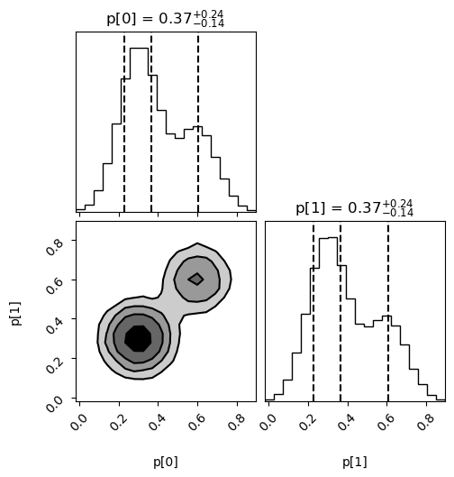
Samples are also useful for making histograms and contour plots of the probability density. For example, the following code uses the corner Python module to create histograms for each parameter, and a contour plot showing their joint distribution:

import corner
import matplotlib.pyplot as plt

corner.corner(
    data=p_samples.T, weights=wgts, labels=['p[0]', 'p[1]'],
    range=[0.999, 0.999], show_titles=True, quantiles=[0.16, 0.5, 0.84],
    plot_datapoints=False, fill_contours=True, smooth=1,
    )
plt.show()

The output, showing the bimodal structure, is:

Parameters:

nbatch (int) – The integrator will return at least nbatch samples drawn from its PDF. The actual number of samples is the smallest multiple of self.last_neval that is equal to or larger than nbatch. Results are packaged in arrays or dictionaries whose elements have an extra index labeling the different samples in the batch. The batch index is the rightmost index if mode='rbatch'; it is the leftmost index if mode is 'lbatch'.
mode (bool) – Batch mode. Allowed modes are 'rbatch' or 'lbatch', corresponding to batch indices that are on the right or the left, respectively. Default is mode='rbatch'.

Returns:

A tuple (wgts,samples) containing samples drawn from the integrator’s PDF, together with their weights wgts. The weighted sample points are distributed through parameter space with a density proportional to the PDF.

In general, samples is either a dictionary or an array depending upon the format of vegas.PDFIntegrator parameter param. For example, if

param = gv.gvar(dict(s='1.5(1)', v=['3.2(8)', '1.1(4)']))

then samples['s'][i] is a sample for parameter p['s'] where index i=0,1...nbatch(approx) labels the sample. The corresponding sample for p['v'][d], where d=0 or 1, is samples['v'][d, i] provided mode='rbatch', which is the default. (Otherwise it is p['v'][i, d], for mode='lbatch'.) The corresponding weight for this sample is wgts[i].

When param is an array, samples is an array with the same shape plus an extra sample index which is either on the right (mode='rbatch', default) or left (mode='lbatch').

Other Objects and Functions¶

class vegas.RAvg(weighted=True, itn_results=None, sum_neval=0, _rescale=True)¶

Running average of scalar-valued Monte Carlo estimates.

This class accumulates independent Monte Carlo estimates (e.g., of an integral) and combines them into a single average. It is derived from gvar.GVar (from the gvar module if it is present) and represents a Gaussian random variable.

Different estimates are weighted by their inverse variances if parameter weight=True; otherwise straight, unweighted averages are used.

Attributes and methods:

mean¶: The mean value of the weighted average.

sdev¶: The standard deviation of the weighted average.

chi2¶: chi**2 of weighted average.

dof¶: Number of degrees of freedom in weighted average.

Q¶: Q or p-value of weighted average’s chi**2.

itn_results¶: A list of the results from each iteration.

sum_neval¶: Total number of integrand evaluations used in all iterations.

add(g)¶: Add estimate g to the running average.

summary(weighted=None)¶

Assemble summary of results, iteration-by-iteration, into a string.

Parameters:: weighted (bool) – Display weighted averages of results from different iterations if True; otherwise show unweighted averages. Default behavior is determined by vegas.

extend(ravg)¶: Merge results from RAvg object ravg after results currently in self.

class vegas.RAvgArray(shape=None, dtype=<class 'object'>, buffer=None, offset=0, strides=None, order=None, weighted=True, itn_results=None, sum_neval=0, rescale=True)¶

Running average of array-valued Monte Carlo estimates.

This class accumulates independent arrays of Monte Carlo estimates (e.g., of an integral) and combines them into an array of averages. It is derived from numpy.ndarray. The array elements are gvar.GVars (from the gvar module if present) and represent Gaussian random variables.

Different estimates are weighted by their inverse covariance matrices if parameter weight=True; otherwise straight, unweighted averages are used.

Attributes and methods:

chi2¶: chi**2 of weighted average.

dof¶: Number of degrees of freedom in weighted average.

Q¶: Q or p-value of weighted average’s chi**2.

itn_results¶: A list of the results from each iteration.

sum_neval¶: Total number of integrand evaluations used in all iterations.

add(g)¶: Add estimate g to the running average.

summary(extended=False, weighted=None)¶

Assemble summary of results, iteration-by-iteration, into a string.

Parameters:

extended (bool) – Include a table of final averages for every component of the integrand if True. Default is False.
weighted (bool) – Display weighted averages of results from different iterations if True; otherwise show unweighted averages. Default behavior is determined by vegas.

extend(ravg)¶: Merge results from RAvgArray object ravg after results currently in self.

class vegas.RAvgDict(dictionary=None, weighted=True, itn_results=None, sum_neval=0, rescale=True)¶

Running average of dictionary-valued Monte Carlo estimates.

This class accumulates independent dictionaries of Monte Carlo estimates (e.g., of an integral) and combines them into a dictionary of averages. It is derived from gvar.BufferDict. The dictionary values are gvar.GVars or arrays of gvar.GVars.

Different estimates are weighted by their inverse covariance matrices if parameter weight=True; otherwise straight, unweighted averages are used.

Attributes and methods:

chi2¶: chi**2 of weighted average.

dof¶: Number of degrees of freedom in weighted average.

Q¶: Q or p-value of weighted average’s chi**2.

itn_results¶: A list of the results from each iteration.

sum_neval¶: Total number of integrand evaluations used in all iterations.

add(g)¶

Augment buffer with data v, indexed by key k.

v is either a scalar or a numpy array (or a list or other data type that can be changed into a numpy.array). If v is a numpy array, it can have any shape.

Same as self[k] = v except when k is already used in self, in which case a ValueError is raised.

summary(extended=False, weighted=None)¶

Assemble summary of results, iteration-by-iteration, into a string.

Parameters:

extended (bool) – Include a table of final averages for every component of the integrand if True. Default is False.
weighted (bool) – Display weighted averages of results from different iterations if True; otherwise show unweighted averages. Default behavior is determined by vegas.

extend(ravg)¶: Merge results from RAvgDict object ravg after results currently in self.

class vegas.PDFEV(results, analyzer=None)¶

Expectation value from vegas.PDFIntegrator.

Expectation values are returned by vegas.PDFIntegrator.__call__() and vegas.PDFIntegrator.stats:

>>> g = gvar.gvar(['1(1)', '10(10)'])
>>> g_ev = vegas.PDFIntegrator(g)
>>> def f(p):
...     return p[0] * p[1]
>>> print(g_ev(f))
10.051(57)
>>> print(g_ev.stats(f))
10(17)

In the first case, the quoted error is the uncertainty in the vegas estimate of the mean of f(p). In the second case, the quoted uncertainty is the standard deviation evaluated with respect to the Gaussian distribution associated with g (added in quadrature to the vegas error, which is negligible here).

vegas.PDFEVs have the following attributes:

pdfnorm¶: Divide PDF by pdfnorm to normalize it.

results¶

Results from the underlying integrals.

Type:: vegas.RAvgDict

In addition, they have all the attributes of the vegas.RAvgDict (results) corresponding to the underlying integrals.

A vegas.PDFEV returned by vegas.PDFIntegrator.stats(self, f...) has three further attributes:

stats¶: An instance of gvar.PDFStatistics containing statistical information about the distribution of f(p).

vegas_mean¶: vegas estimate for the mean value of f(p). The uncertainties in vegas_mean are the integration errors from vegas.

vegas_cov¶: vegas estimate for the covariance matrix of f(p). The uncertainties in vegas_cov are the integration errors from vegas.

vegas_sdev¶: vegas estimate for the standard deviation of f(p). The uncertainties in vegas_sdev are the integration errors from vegas.

class vegas.PDFEVArray(results, analyzer=None)¶

Array of expectation values from vegas.PDFIntegrator.

Expectation values are returned by vegas.PDFIntegrator.__call__() and vegas.PDFIntegrator.stats:

>>> g = gvar.gvar(['1(1)', '10(10)'])
>>> g_ev = vegas.PDFIntegrator(g)
>>> def f(p):
...     return [p[0], p[1], p[0] * p[1]]
>>> print(g_ev(f))
[0.9992(31) 10.024(29) 10.051(57)]
>>> print(g_ev.stats(f))
[1.0(1.0) 10(10) 10(17)]

In the first case, the quoted errors are the uncertainties in the vegas estimates of the means. In the second case, the quoted uncertainties are the standard deviations evaluated with respect to the Gaussian distribution associated with g (added in quadrature to the vegas errors, which are negligible here).

vegas.PDFEVArrays have the following attributes:

pdfnorm¶: Divide PDF by pdfnorm to normalize it.

results¶

Results from the underlying integrals.

Type:: vegas.RAvgDict

In addition, they have all the attributes of the vegas.RAvgDict (results) corresponding to the underlying integrals.

A vegas.PDFEVArray s returned by vegas.PDFIntegrator.stats(self, f...) has three further attributes:

stats¶: s.stats[i] is a gvar.PDFStatistics object containing statistical information about the distribution of f(p)[i].

vegas_mean¶: vegas estimates for the mean values of f(p). The uncertainties in vegas_mean are the integration errors from vegas.

vegas_cov¶: vegas estimate for the covariance matrix of f(p). The uncertainties in vegas_cov are the integration errors from vegas.

vegas_sdev¶: vegas estimate for the standard deviation of f(p). The uncertainties in vegas_sdev are the integration errors from vegas.

class vegas.PDFEVDict(results, analyzer=None)¶

Dictionary of expectation values from vegas.PDFIntegrator.

Expectation values are returned by vegas.PDFIntegrator.__call__() and vegas.PDFIntegrator.stats:

>>> g = gvar.gvar(['1(1)', '10(10)'])
>>> g_ev = vegas.PDFIntegrator(g)
>>> def f(p):
...     return dict(p=p, prod=p[0] * p[1])
>>> print(g_ev(f))
{'p': array([0.9992(31), 10.024(29)], dtype=object), 'prod': 10.051(57)}
>>> print(g_ev.stats(f))
{'p': array([1.0(1.0), 10(10)], dtype=object), 'prod': 10(17)}

In the first case, the quoted errors are the uncertainties in the vegas estimates of the means. In the second case, the quoted uncertainties are the standard deviations evaluated with respect to the Gaussian distribution associated with g (added in quadrature to the vegas errors, which are negligible here).

vegas.PDFEVDict objects have the following attributes:

pdfnorm¶: Divide PDF by pdfnorm to normalize it.

results¶

Results from the underlying integrals.

Type:: vegas.RAvgDict

In addition, they have all the attributes of the vegas.RAvgDict (results) corresponding to the underlying integrals.

A vegas.PDFEVDict object s returned by vegas.PDFIntegrator.stats() has three further attributes:

stats¶: s.stats[k] is a gvar.PDFStatistics object containing statistical information about the distribution of f(p)[k].

vegas_mean¶: vegas estimates for the mean values of f(p). The uncertainties in vegas_mean are the integration errors from vegas.

vegas_cov¶: vegas estimate for the covariance matrix of f(p). The uncertainties in vegas_cov are the integration errors from vegas.

vegas_sdev¶: vegas estimate for the standard deviation of f(p). The uncertainties in vegas_sdev are the integration errors from vegas.

vegas.lbatchintegrand(f)¶

Decorator for batch integrand functions.

Applying vegas.lbatchintegrand() to a function fcn repackages the function in a format that vegas can understand. Appropriate functions take a numpy array of integration points x[i, d] as an argument, where i=0... labels the integration point and d=0... labels direction, and return an array f[i] of integrand values (or arrays of integrand values) for the corresponding points. The meaning of fcn(x) is unchanged by the decorator.

An example is

import vegas
import numpy as np

@vegas.lbatchintegrand      # or @vegas.lbatchintegrand
def f(x):
    return np.exp(-x[:, 0] - x[:, 1])

for the two-dimensional integrand $\exp(-x_0 - x_1)$ . When integrands have dictionary arguments xd, each element of the dictionary has an extra index (on the left): xd[key][:, ...].

vegas.batchintegrand() is the same as vegas.lbatchintegrand().

class vegas.LBatchIntegrand¶

Wrapper for lbatch integrands.

Used by vegas.lbatchintegrand().

vegas.LBatchIntegrand is the same as vegas.BatchIntegrand.

vegas.rbatchintegrand(f)¶: Same as vegas.lbatchintegrand() but with batch indices on the right (not left).

class vegas.RBatchIntegrand¶: Same as vegas.LBatchIntegrand but with batch indices on the right (not left).

vegas.ravg(reslist, weighted=None, rescale=None)¶

Create running average from list of vegas results.

This function is used to change how the weighted average of vegas results is calculated. For example, the following code discards the first five results (where vegas is still adapting) and does an unweighted average of the last five:

import vegas

def fcn(p):
    return p[0] * p[1] * p[2] * p[3] * 16.

itg = vegas.Integrator(4 * [[0,1]])
r = itg(fcn)
print(r.summary())
ur = vegas.ravg(r.itn_results[5:], weighted=False)
print(ur.summary())

The unweighted average can be useful because it is unbiased. The output is:

itn   integral        wgt average     chi2/dof        Q
-------------------------------------------------------
 1.013(19)       1.013(19)           0.00     1.00
 0.997(14)       1.002(11)           0.45     0.50
 1.021(12)       1.0112(80)          0.91     0.40
 0.9785(97)      0.9980(62)          2.84     0.04
 1.0067(85)      1.0010(50)          2.30     0.06
 0.9996(75)      1.0006(42)          1.85     0.10
 1.0020(61)      1.0010(34)          1.54     0.16
 1.0051(52)      1.0022(29)          1.39     0.21
 1.0046(47)      1.0029(24)          1.23     0.27
 0.9976(47)      1.0018(22)          1.21     0.28

itn   integral        average         chi2/dof        Q
-------------------------------------------------------
 0.9996(75)      0.9996(75)          0.00     1.00
 1.0020(61)      1.0008(48)          0.06     0.81
 1.0051(52)      1.0022(37)          0.19     0.83
 1.0046(47)      1.0028(30)          0.18     0.91
 0.9976(47)      1.0018(26)          0.31     0.87

Parameters:

reslist (list) – List whose elements are gvar.GVars, arrays of gvar.GVars, or dictionaries whose values are gvar.GVars or arrays of gvar.GVars. Alternatively reslist can be the object returned by a call to a vegas.Integrator object (i.e, an instance of any of vegas.RAvg, vegas.RAvgArray, vegas.RAvgArray, vegas.PDFEV, vegas.PDFEVArray, vegas.PDFEVArray).
weighted (bool) – Running average is weighted (by the inverse covariance matrix) if True. Otherwise the average is unweighted, which makes most sense if reslist items were generated by vegas with little or no adaptation (e.g., with adapt=False). If weighted is not specified (or is None), it is set equal to getattr(reslist, 'weighted', True).
rescale – Integration results are divided by rescale before taking the weighted average if weighted=True; otherwise rescale is ignored. Setting rescale=True is equivalent to setting rescale=reslist[-1]. If rescale is not specified (or is None), it is set equal to getattr(reslist, 'rescale', True).

`vegas` Module¶

Introduction¶

Integrator Objects¶

AdaptiveMap Objects¶

PDFIntegrator Objects¶

Other Objects and Functions¶

Table of Contents

Previous topic

This Page

vegas Module¶

Introduction¶

Integrator Objects¶

AdaptiveMap Objects¶

PDFIntegrator Objects¶

Other Objects and Functions¶

`vegas` Module¶