Tutorial¶

Introduction¶

Class vegas.Integrator gives Monte Carlo estimates of arbitrary multidimensional integrals using the vegas algorithm (G. P. Lepage, J. Comput. Phys. 27 (1978) 192 and J. Comput. Phys. 439 (2021) 110386). The algorithm has two components. First an automatic transformation is applied to to the integration variables in an attempt to flatten the integrand. Then a Monte Carlo estimate of the integral is made using the transformed variables. Flattening the integrand makes the integral easier and improves the estimate. The transformation applied to the integration variables is optimized over several iterations of the algorithm: information about the integrand that is collected during one iteration is used to improve the transformation used in the next iteration.

Monte Carlo integration makes few assumptions about the integrand — it needn’t be analytic nor even continuous. This makes Monte Carlo integration unusually robust. It also makes it well suited for adaptive integration. Adaptive strategies are essential for multidimensional integration, especially in high dimensions, because multidimensional space is large, with lots of corners, making it easy to lose important features in the integrand.

Monte Carlo integration also provides efficient and reliable methods for estimating the accuracy of its results. In particular, each Monte Carlo estimate of an integral is a random number from a distribution whose mean is the correct value of the integral. This distribution is Gaussian or normal provided the number of integrand samples is sufficiently large. In practice we generate multiple estimates of the integral in order to verify that the distribution is indeed Gaussian. Error analysis is straightforward if the integral estimates are Gaussian.

The vegas algorithm has been in use for decades and implementations are available in many programming languages, including Fortran (the original version), C and C++. The algorithm used here is significantly improved over the original implementation, and that used in most other implementations. It uses two adaptive strategies: importance sampling, as in the original implementation, and adaptive stratified sampling, which is new. The new algorithm is described in G. P. Lepage, arXiv_2009.05112 (J. Comput. Phys. 439 (2021) 110386).

This module is written in Cython, so it is almost as fast as compiled Fortran or C, particularly when the integrand is also coded in Cython (or some other compiled language), as discussed below.

The following sections describe how to use vegas. Almost every example shown is a complete code, which can be copied into a file and run with Python. It is worthwhile playing with the parameters to see how things change.

About Printing: The examples in this tutorial use the print function as it is used in Python 3. Drop the outermost parenthesis in each print statement if using Python 2, or add

from __future__ import print_function

at the start of your file.

Basic Integrals¶

Here we illustrate the use of vegas by estimating the integral

$C\int_{-1}^1 dx_0 \int_0^1 dx_1 \int_0^1 dx_2 \int_0^1 dx_3 \,\,\mathrm{e}^{- 100 \sum_{d}(x_d-0.5)^2} ,$

where constant $C$ is chosen so that the exact integral is 1. The following code shows how this can be done:

import vegas
import math

def f(x):
    dx2 = 0
    for d in range(4):
        dx2 += (x[d] - 0.5) ** 2
    return math.exp(-dx2 * 100.) * 1013.2118364296088

integ = vegas.Integrator([[-1, 1], [0, 1], [0, 1], [0, 1]])

result = integ(f, nitn=10, neval=1000)
print(result.summary())
print('result = %s    Q = %.2f' % (result, result.Q))

First we define the integrand f(x) where x[d] specifies a point in the 4-dimensional space. We then create an integrator, integ, which is an integration operator that can be applied to any 4-dimensional function. It is where we specify the integration volume. Finally we apply integ to our integrand f(x), telling the integrator to estimate the integral using nitn=10 iterations of the vegas algorithm, each of which uses no more than neval=1000 evaluations of the integrand. Each iteration produces an independent estimate of the integral. The final estimate is the weighted average of the results from all 10 iterations, and is returned by integ(f ...). The call result.summary() returns a summary of results from each iteration.

This code produces the following output:

itn   integral        wgt average     chi2/dof        Q
-------------------------------------------------------
 2.6(1.4)        2.6(1.4)            0.00     1.00
 1.32(25)        1.36(25)            0.75     0.39
 0.909(96)       0.968(89)           1.79     0.17
 1.039(69)       1.012(55)           1.32     0.26
 0.929(34)       0.952(29)           1.41     0.23
 1.003(26)       0.980(19)           1.47     0.20
 0.994(18)       0.988(13)           1.27     0.27
 0.998(14)       0.9922(98)          1.13     0.34
 1.020(12)       1.0035(75)          1.39     0.20
 1.011(12)       1.0057(64)          1.27     0.25

result = 1.0057(64)    Q = 0.25

There are several things to note here:

Adaptation: Integration estimates are shown for each of the 10 iterations, giving both the estimate from just that iteration, and the weighted average of results from all iterations up to that point. The estimates from the first two iterations are not accurate at all, with errors equal to 25–140% of the final result. vegas initially has no information about the integrand and so does a relatively poor job of estimating the integral. It uses information from the samples in one iteration, however, to remap the integration variables for subsequent iterations, concentrating samples where the function is largest and reducing errors. As a result, the per-iteration error is reduced to 3.4% by the fifth iteration, and almost to 1% by the end — an improvement by a factor of more than 100 from the start. Eventually the per-iteration error stops decreasing because vegas has found the optimal remapping, at which point it is fully adapted to the integrand.

Weighted Average: The final result, 1.0057 ± 0.0064, is obtained from a weighted average of the separate results from each iteration: estimates are weighted by the inverse variance, thereby giving much less weight to the early iterations, where the errors are largest. The individual estimates are statistical: each is a random number drawn from a distribution whose mean equals the correct value of the integral, and the errors quoted are estimates of the standard deviations of those distributions. The distributions are Gaussian provided the number of integrand evaluations per iteration (neval) is sufficiently large, in which case the standard deviation is a reliable estimate of the error. The weighted average $\overline I$ minimizes

$\chi^2 \,\equiv\, \sum_i \frac{(I_i - \overline I)^2}{\sigma_{i}^2}$

where $I_i \pm \sigma_{i}$ are the estimates from individual iterations. If the $I_i$ are Gaussian, $\chi^2$ should be of order the number of degrees of freedom (plus or minus the square root of double that number); here the number of degrees of freedom is the number of iterations minus 1.

The distributions are likely non-Gaussian, and error estimates unreliable, if $\chi^2$ is much larger than the number of iterations. This criterion is quantified by the Q or p-value of the $\chi^2$ , which is the probability that a larger $\chi^2$ could result from random (Gaussian) fluctuations. A very small Q (less than 0.05-0.1) indicates that the $\chi^2$ is too large to be accounted for by statistical fluctuations — that is, the estimates of the integral from different iterations do not agree with each other to within errors. This means that neval is not sufficiently large to guarantee Gaussian behavior, and must be increased if the error estimates are to be trusted.

integ(f...) returns a weighted-average object, of type vegas.RAvg, that has the following attributes:

result.mean — weighted average of all estimates of the integral;

result.sdev — standard deviation of the weighted average;

result.chi2 — $\chi^2$ of the weighted average;

result.dof — number of degrees of freedom;

result.Q — Q or p-value of the weighted average’s $\chi^2$ ;

result.itn_results — list of the integral estimates from each iteration;

result.sum_neval — total number of integrand evaluations used.

result.avg_neval — average number of integrand evaluations per iteration

In this example the final Q is 0.25, indicating that the $\chi^2$ for this average is not particularly unlikely and thus the error estimate is likely reliable.

Precision: The precision of vegas estimates is determined by nitn, the number of iterations of the vegas algorithm, and by neval, the maximum number of integrand evaluations made per iteration. The computing cost is typically proportional to the product of nitn and neval. The number of integrand evaluations per iteration varies from iteration to iteration, here between 860 and 960. Typically vegas needs more integration points in early iterations, before it has fully adapted to the integrand.

We can increase precision by increasing either nitn or neval, but it is generally far better to increase neval. For example, adding the following lines to the code above
result = integ(f, nitn=100, neval=1000)
print('larger nitn  => %s    Q = %.2f' % (result, result.Q))

result = integ(f, nitn=10, neval=1e4)
print('larger neval => %s    Q = %.2f' % (result, result.Q))
generates the following results:
larger nitn  => 1.0003(13)    Q = 0.79
larger neval => 0.99981(53)    Q = 0.28
The total number of integrand evaluations, nitn * neval, is about the same in both cases, but increasing neval is more than twice as accurate as increasing nitn. Typically you want to use no more than 10 or 20 iterations beyond the point where vegas has fully adapted. You want some number of iterations so that you can verify Gaussian behavior by checking the $\chi^2$ and Q, but not too many.

It is also generally useful to compare two or more results from values of neval that differ by a significant factor (4–10, say). These should agree within errors. If they do not, it could be due to non-Gaussian artifacts caused by a small neval. vegas estimates have two sources of error. One is the statistical error, which is what is quoted by vegas. The other is a systematic error due to residual non-Gaussian effects. The systematic error vanishes like 1/neval or faster, and so becomes negligible compared with the statistical error as neval increases. The systematic error can bias the Monte Carlo estimate, however, if neval is insufficiently large. This usually results in a large $\chi^2$ (and small Q), but a more reliable check is to compare results that use significantly different values of neval. The systematic errors due to non-Gaussian behavior are likely negligible if the different estimates agree to within the statistical errors.

The possibility of systematic biases is another reason for increasing neval rather than nitn to obtain more precision. Making neval larger and larger is guaranteed to improve the Monte Carlo estimate, as the statistical error decreases and the systematic error decreases even more quickly. Making nitn larger and larger, on the other hand, is guaranteed eventually to give the wrong answer. This is because at some point the statistical error (which falls as sqrt(1/nitn)) will no longer mask the systematic error (which is unaffected by nitn). The systematic error for the integral above (with neval=1000) is about -0.0008, which is negligible compared to the statistical error unless nitn is of order 1500 or larger — so systematic errors aren’t a problem with nitn=10.

Early Iterations: Integral estimates from early iterations, before vegas has adapted, can be quite crude. With very peaky integrands, these are often far from the correct answer with highly unreliable error estimates. For example, the integral above becomes more difficult if we double the length of each side of the integration volume by redefining integ as:
integ = vegas.Integrator([[-2, 2], [0, 2], [0, 2], [0., 2]])
The code above then gives:
itn   integral        wgt average     chi2/dof        Q
-------------------------------------------------------
  1   0.0011(10)      0.0011(10)          0.00     1.00
  2   0.074(56)       0.0011(10)          1.71     0.19
  3   0.250(59)       0.0012(10)          9.65     0.00
  4   0.93(14)        0.0013(10)         21.40     0.00
  5   0.874(70)       0.0015(10)         54.87     0.00
  6   0.949(39)       0.0021(10)        162.08     0.00
  7   0.949(30)       0.0033(10)        301.18     0.00
  8   0.985(25)       0.0050(10)        484.50     0.00
  9   0.967(19)       0.0078(10)        738.53     0.00
 10   0.988(15)       0.0125(10)       1131.46     0.00

result = 0.0125(10)    Q = 0.00
vegas misses the peak completely in the first iteration, giving an estimate that is completely wrong (by 1000 standard deviations!). Some of its samples hit the peak’s shoulders, so vegas is eventually able to find the peak (by iterations 5–6), but the integrand estimates are wildly non-Gaussian before that point. This results in a nonsensical final result, as indicated by the Q = 0.00.

It is common practice in using vegas to discard estimates from the first several iterations, before the algorithm has adapted, in order to avoid ruining the final result in this way. This is done by replacing the single call to integ(f...) in the original code with two calls:
# step 1 -- adapt to f; discard results
integ(f, nitn=10, neval=1000)

# step 2 -- integ has adapted to f; keep results
result = integ(f, nitn=10, neval=1000)
print(result.summary())
print('result = %s    Q = %.2f' % (result, result.Q))
The integrator is trained in the first step, as it adapts to the integrand, and so is more or less fully adapted from the start in the second step, which yields:
itn   integral        wgt average     chi2/dof        Q
-------------------------------------------------------
  1   0.993(17)       0.993(17)           0.00     1.00
  2   1.062(48)       1.001(16)           1.83     0.18
  3   0.964(20)       0.987(13)           1.91     0.15
  4   0.974(16)       0.9817(99)          1.40     0.24
  5   0.990(15)       0.9843(82)          1.10     0.35
  6   1.012(16)       0.9899(73)          1.34     0.25
  7   0.999(15)       0.9917(65)          1.16     0.32
  8   1.008(12)       0.9953(58)          1.20     0.30
  9   1.013(15)       0.9977(54)          1.20     0.29
 10   0.983(14)       0.9958(50)          1.17     0.31

result = 0.9958(50)    Q = 0.31
The final result is now reliable.

Other Integrands: Once integ has been trained on f(x), it can be usefully applied to other functions with similar structure. For example, adding the following at the end of the original code,
def g(x):
    return x[0] * f(x)

result = integ(g, nitn=10, neval=1000)
print(result.summary())
print('result = %s    Q = %.2f' % (result, result.Q))
gives the following new output:
itn   integral        wgt average     chi2/dof        Q
-------------------------------------------------------
  1   0.4933(61)      0.4933(61)          0.00     1.00
  2   0.5017(54)      0.4980(40)          1.04     0.31
  3   0.4975(64)      0.4979(34)          0.52     0.59
  4   0.5059(60)      0.4998(30)          0.80     0.49
  5   0.5075(64)      0.5012(27)          0.90     0.46
  6   0.4907(66)      0.4997(25)          1.15     0.33
  7   0.5009(47)      0.5000(22)          0.97     0.45
  8   0.5082(58)      0.5010(21)          1.08     0.38
  9   0.5016(63)      0.5010(20)          0.94     0.48
 10   0.4934(76)      0.5006(19)          0.94     0.49

result = 0.5006(19)    Q = 0.49
Again the grid is almost optimal for g(x) from the start, because g(x) peaks in the same region as f(x). The exact value for this integral is very close to 0.5.

Non-Rectangular Volumes: vegas can integrate over volumes of non-rectangular shape. For example, we can replace integrand f(x) above by the same Gaussian, but restricted to a 4-sphere of radius 0.2, centered on the Gaussian:
import vegas
import math

def f_sph(x):
    dx2 = 0
    for d in range(4):
        dx2 += (x[d] - 0.5) ** 2
    if dx2 < 0.2 ** 2:
        return math.exp(-dx2 * 100.) * 1115.3539360527281318
    else:
        return 0.0

integ = vegas.Integrator([[-1, 1], [0, 1], [0, 1], [0, 1]])

integ(f_sph, nitn=10, neval=1000)           # adapt the grid
result = integ(f_sph, nitn=10, neval=1000)  # estimate the integral
print(result.summary())
print('result = %s    Q = %.2f' % (result, result.Q))
The normalization is adjusted to again make the exact integral equal 1. Integrating as before gives:
itn   integral        wgt average     chi2/dof        Q
-------------------------------------------------------
  1   0.992(20)       0.992(20)           0.00     1.00
  2   0.993(19)       0.992(14)           0.00     0.97
  3   1.002(18)       0.996(11)           0.09     0.91
  4   1.004(22)       0.9973(98)          0.10     0.96
  5   1.026(30)       1.0001(93)          0.28     0.89
  6   1.053(92)       1.0007(93)          0.29     0.92
  7   1.035(30)       1.0038(89)          0.45     0.85
  8   0.991(19)       1.0014(80)          0.44     0.88
  9   0.968(18)       0.9956(73)          0.76     0.64
 10   1.022(37)       0.9966(72)          0.73     0.68

result = 0.9966(72)    Q = 0.68
It is a good idea to make the actual integration volume as large a fraction as possible of the total volume used by vegas — by choosing integration variables properly — so vegas doesn’t spend lots of effort on regions where the integrand is exactly 0. Also, it can be challenging for vegas to find the region of non-zero integrand in high dimensions: integrating f_sph(x) in 20 dimensions instead of 4, for example, would require neval=1e16 integrand evaluations per iteration to have any chance of finding the region of non-zero integrand, because the volume of the 20-dimensional sphere is a tiny fraction of the total integration volume. The final error in the example above would have been cut in half had we used the integration volume 4 * [[0.3, 0.7]] instead of [[-1, 1], [0, 1], [0, 1], [0, 1]].

Note, finally, that integration to infinity is also possible: map the relevant variable into a different variable of finite range. For example, an integral over $x\equiv b z / (1-z)$ from 0 to infinity is easily re-expressed as an integral over $z$ from 0 to 1, where the transformation emphasizes the region in $x$ of order free parameter $b$ .

Damping: The result in the previous section can be improved somewhat by slowing down vegas’s adaptation:
...
integ(f_sph, nitn=10, neval=1000, alpha=0.1)
result = integ(f_sph, nitn=10, neval=1000, alpha=0.1)
...
Parameter alpha controls the speed with which vegas adapts, with smaller alphas giving slower adaptation. Here we reduce alpha to 0.1, from its default value of 0.5, and get the following output:
itn   integral        wgt average     chi2/dof        Q
-------------------------------------------------------
  1   1.008(26)       1.008(26)           0.00     1.00
  2   0.993(23)       0.999(17)           0.19     0.66
  3   1.005(21)       1.002(13)           0.11     0.89
  4   1.016(20)       1.006(11)           0.19     0.91
  5   0.973(18)       0.9967(95)          0.73     0.57
  6   1.016(18)       1.0009(84)          0.77     0.57
  7   1.008(18)       1.0023(76)          0.66     0.68
  8   0.990(17)       1.0002(69)          0.63     0.73
  9   1.008(17)       1.0012(64)          0.58     0.80
 10   0.958(17)       0.9959(60)          1.12     0.34

result = 0.9959(60)    Q = 0.34
Notice how the errors fluctuate less from iteration to iteration with the smaller alpha in this case. Persistent, large fluctuations in the size of the per-iteration errors is often a signal that alpha should be reduced. With larger alphas, vegas can over-react to random fluctuations it encounters as it samples the integrand.

In general, we want alpha to be large enough so that vegas adapts quickly to the integrand, but not so large that it has difficulty holding on to the optimal tuning once it has found it. The best value depends upon the integrand.

adapt=False: Adaptation can be turned off completely by setting parameter adapt=False. There are three reasons one might do this. The first is if vegas is exhibiting the kind of instability discussed in the previous section — one might use the following code, instead of that presented there:
...
integ(f_sph, nitn=10, neval=1000, alpha=0.1)
result = integ(f_sph, nitn=10, neval=1000, adapt=False)
...
The second reason is that vegas runs slightly faster when it is no longer adapting to the integrand. The difference is not signficant for complicated integrands, but is noticable in simpler cases.

The third reason for turning off adaptation is that vegas uses unweighted averages, rather than weighted averages, to combine results from different iterations when adapt=False. Unweighted averages are not biased. They have no systematic error of the sort discussed above, and so give correct results even for very large numbers of iterations, nitn.

The lack of systematic biases is not a strong reason for turning off adaptation, however, since the biases are usually negligible (see above). The most important reason is the first: stability.

adapt=False is particularly useful when the number of integrand evaluations neval is small for the integrand, leading to large fluctuations in the errors from iteration to iteration. For example, the following output is from an estimate (with neval=2.5e4) of an eight-dimensional integral with three sharp peaks along the diagonal (Eq. (45) in arXiv_2009.05112, normalized so that the correct answer equals 1):
itn   integral        wgt average     chi2/dof        Q
-------------------------------------------------------
 1   0.75(43)        0.75(43)            0.00     1.00
 2   0.506(58)       0.510(58)           0.32     0.57
 3   0.80(21)        0.530(56)           1.02     0.36
 4   0.76(11)        0.576(50)           1.81     0.14
 5   1.27(29)        0.596(49)           2.74     0.03
 6   1.10(19)        0.629(48)           3.56     0.00
 7   0.802(73)       0.681(40)           3.63     0.00
 8   2.8(2.0)        0.681(40)           3.27     0.00
 9   0.907(90)       0.719(36)           3.52     0.00
10   1.07(16)        0.736(35)           3.65     0.00

itn   integral        average         chi2/dof        Q
-------------------------------------------------------
 1   1.13(14)        1.13(14)            0.00     1.00
 2   1.064(96)       1.095(86)           0.13     0.72
 3   1.03(10)        1.072(67)           0.19     0.83
 4   0.924(94)       1.035(55)           0.58     0.63
 5   0.858(71)       1.000(46)           1.08     0.37
 6   0.97(11)        0.995(43)           0.84     0.52
 7   0.924(69)       0.985(38)           0.84     0.54
 8   1.19(16)        1.010(39)           1.01     0.42
 9   1.74(73)        1.092(88)           1.01     0.42
10   0.942(89)       1.077(80)           1.02     0.42
The first 10 iterations are used to train the vegas map; their results are discarded. The next 10 iterations, with adapt=False, have uncertainties that fluctuate in size by an order of magnitude, but still give a reliable estimate for the integral (1.08(8)). Allowing vegas to continue adapting in the the second set of iterations gives results like 0.887(25), which is 4.5 standard deviations too low; the real uncertainty is larger than ±0.025.

Training the integrator and then setting adapt=False for the final results works best if the number of evaluations per iteration (neval) is the same in both steps. This is because the second of vegas’s adaptation strategies (Adaptive Stratified Sampling) is usually reinitialized when neval changes, and so is not used at all when neval is changed at the same time adapt=False is set.

Multiple Integrands Simultaneously¶

vegas can be used to integrate multiple integrands simultaneously, using the same integration points for each of the integrands. This is useful in situations where the integrands have similar structure, with peaks in the same locations. There can be signficant advantages in sampling different integrands at precisely the same points in x space, because then Monte Carlo estimates for the different integrals are correlated. If the integrands are very similar to each other, the correlations can be very strong. This leads to greatly reduced errors in ratios or differences of the resulting integrals as the fluctuations cancel.

Consider a simple example. We want to compute the normalization and first two moments of a sharply peaked probability distribution:

$I_0 &\equiv \int_0^1 d^4x\; \mathrm{e}^{- 200 \sum_{d}(x_d-0.5)^2}\\ I_1 &\equiv \int_0^1 d^4x\; x_0 \; \mathrm{e}^{- 200 \sum_{d}(x_d-0.5)^2} \\ I_2 &\equiv \int_0^1 d^4x\; x_0^2 \; \mathrm{e}^{- 200 \sum_{d}(x_d-0.5)^2}$

From these integrals we determine the mean and width of the distribution projected onto one of the axes:

$\langle x \rangle &\equiv I_1 / I_0 \\[1ex] \sigma_x^2 &\equiv \langle x^2 \rangle - \langle x \rangle^2 \\ &= I_2 / I_0 - (I_1 / I_0)^2$

This can be done using the following code:

import vegas
import math
import gvar as gv

def f(x):
    dx2 = 0.0
    for d in range(4):
        dx2 += (x[d] - 0.5) ** 2
    f = math.exp(-200 * dx2)
    return [f, f * x[0], f * x[0] ** 2]

integ = vegas.Integrator(4 * [[0, 1]])

# adapt grid
training = integ(f, nitn=10, neval=2000)

# final analysis
result = integ(f, nitn=10, neval=10000)
print('I[0] =', result[0], '  I[1] =', result[1], '  I[2] =', result[2])
print('Q = %.2f\n' % result.Q)
print('<x> =', result[1] / result[0])
print(
    'sigma_x**2 = <x**2> - <x>**2 =',
    result[2] / result[0] - (result[1] / result[0]) ** 2
    )
print('\ncorrelation matrix:\n', gv.evalcorr(result))

The code is very similar to that used in the previous section. The main difference is that the integrand function and vegas return arrays of results — in both cases, one result for each of the three integrals. vegas always adapts to the first integrand in the array. The Q value is for all three of the integrals, taken together.

The code produces the following output:

I[0] = 0.00024682(12)   I[1] = 0.000123417(61)   I[2] = 0.000062327(33)
Q = 0.93

<x> = 0.500017(49)
sigma_x**2 = <x**2> - <x>**2 = 0.0024983(73)

correlation matrix:
 [[1.         0.98002885 0.92558296]
 [0.98002885 1.         0.98157932]
 [0.92558296 0.98157932 1.        ]]

The estimates for the individual integrals are separately accurate to about ±0.05%, but the estimate for $\langle x \rangle = I_1/I_0$ is accurate to ±0.01%. This is almost an order of magnitude (8x) more accurate than we would obtain absent correlations. The correlation matrix shows that there is 98% correlation between the statistical fluctuations in estimates for $I_0$ and $I_1$ , and so the bulk of these fluctuations cancel in the ratio. The estimate for the variance $\sigma^2_x$ is 48x more accurate than we would have obtained had the integrals been evaluated separately. Both estimates are correct to within the quoted errors.

The individual results are objects of type gvar.GVar, which represent Gaussian random variables. Such objects have means (result[i].mean) and standard deviations (result[i].sdev), but also can be statistically correlated with other gvar.GVars. Such correlations are handled automatically by gvar when gvar.GVars are combined with each other or with numbers in arithmetical expressions. (Documentation for gvar can be found at https://gvar.readthedocs.io or with the source code at https://github.com/gplepage/gvar.git.)

Dictionaries¶

Integrands can return dictionaries instead of arrays. The example in the previous section, for example, can be rewritten as

import vegas
import math
import gvar as gv

def f(x):
    dx2 = 0.0
    for d in range(4):
        dx2 += (x[d] - 0.5) ** 2
    f = math.exp(-200 * dx2)
    return {'1':f, 'x':f * x[0], 'x**2':f * x[0] ** 2}

integ = vegas.Integrator(4 * [[0, 1]])

# adapt grid
training = integ(f, nitn=10, neval=2000)

# final analysis
result = integ(f, nitn=10, neval=10000)
print(result)
print('Q = %.2f\n' % result.Q)
print('<x> =', result['x'] / result['1'])
print(
    'sigma_x**2 = <x**2> - <x>**2 =',
    result['x**2'] / result['1'] - (result['x'] / result['1']) ** 2
    )

which returns the following output:

{'1': 0.00024682(12),'x': 0.000123417(61),'x**2': 0.000062327(33)}
Q = 0.93

<x> = 0.500017(49)
sigma_x**2 = <x**2> - <x>**2 = 0.0024983(73)

The result returned by vegas is a dictionary using the same keys as the dictionary returned by the integrand. Using a dictionary with descriptive keys, instead of an array, can often make code more intelligible, and, therefore, easier to write and maintain. Here the values in the integrand’s dictionary are all numbers; in general, values can be either numbers or arrays (of any shape).

Dictionaries can also be used for the integration variables. For example, the following code calculates the volume of a unit sphere using spherical coordinates:

import numpy as np
import vegas

def f(xd):
    r = xd['r']
    theta = xd['theta']
    phi = xd['phi']
    return r ** 2 * np.sin(theta)

integ = vegas.Integrator(dict(r=(0,1), theta=(0, np.pi), phi=(0, 2 * np.pi)))
volume = integ(f, neval=1000, nitn=10)
print(volume)

Running this code gives a result of 4.1852(44) which agrees well (0.1%) with the correct result $4\pi/3$ . This can be generalized to DIM dimensions, where now xd['phi'] is an array of variables: e.g.,

import numpy as np
import vegas

DIM = 5

def f(xd):
    r = xd['r']
    phi = xd['phi']
    # construct Euclidean coordinates, Jacobian
    x = np.zeros(DIM, float)
    x[:] = r
    x[1:] *= np.cumprod(np.sin(phi), axis=0)
    jac = np.prod(x[1:-1], axis=0) * r
    x[:-1] *= np.cos(phi)
    # calculate contribution to sphere's volume
    return jac

integ = vegas.Integrator(dict(
    r=(0,1),
    phi=(DIM - 2) * [(0, np.pi)] + [(0, 2 * np.pi)]
    ))
warmup = integ(f, neval=1000, nitn=10)
volume = integ(f, neval=1000, nitn=10)
print(integ.settings(), '\n')
print(f'volume(dim={DIM}) = {volume}')

This code generates the following output:

Integrator Settings:
    1000 (approx) integrand evaluations in each of 10 iterations
    number of: strata/axis = [3 3 3 2 2]
               increments/axis = [ 99  99  99 100 100]
               h-cubes = 108  processors = 1
               evaluations/batch >= 5e+04
               2 <= evaluations/h-cube <= 5e+04
    minimize_mem = False  adapt_to_errors = False  adapt = True
    accuracy: relative = 0  absolute = 0
    damping: alpha = 0.5  beta= 0.75

    key/index    axis          integration limits
    ---------------------------------------------
            r       0                  (0.0, 1.0)
        phi 0       1    (0.0, 3.141592653589793)
            1       2    (0.0, 3.141592653589793)
            2       3    (0.0, 3.141592653589793)
            3       4    (0.0, 6.283185307179586)
 

volume(dim=5) = 5.254(12)

Calculating Distributions¶

vegas is often used to calculate distributions. The following code, for example, evaluates both an integral I and the contributions dI to the integral coming from each of five different intervals dr in the radius measured from the center of the integration volume. The normalized contributions dI/I are then tabulated:

import vegas
import numpy as np

RMAX = (2 * 0.5**2) ** 0.5

def fcn(x):
    dx2 = 0.0
    for d in range(2):
        dx2 += (x[d] - 0.5) ** 2
    I = np.exp(-dx2)
    # add I to appropriate bin in dI
    dI = np.zeros(5, dtype=float)
    dr = RMAX / len(dI)
    j = int(dx2 ** 0.5 / dr)
    dI[j] = I
    return dict(I=I, dI=dI)

integ = vegas.Integrator(2 * [(0,1)])

# results returned in a dictionary
result = integ(fcn)
print(result.summary())
print('   I =', result['I'])
print('dI/I =', result['dI'] / result['I'])
print('sum(dI/I) =', sum(result['dI']) / result['I'])

Note the check at the end, to verify that the sum of the dI[i]s equals the original integral. Running this script gives the following output:

itn   integral        wgt average     chi2/dof        Q
-------------------------------------------------------
  1   0.85040(55)     0.85040(55)         0.00     1.00
  2   0.85039(45)     0.85040(35)         0.76     0.60
  3   0.85085(39)     0.85061(26)         0.63     0.82
  4   0.85105(33)     0.85079(20)         0.52     0.95
  5   0.85105(30)     0.85087(17)         0.60     0.94
  6   0.85097(24)     0.85091(14)         0.55     0.98
  7   0.85099(21)     0.85096(11)         0.72     0.90
  8   0.85112(17)     0.851013(93)        0.66     0.95
  9   0.85114(15)     0.851053(79)        0.70     0.94
 10   0.85101(13)     0.851041(67)        0.68     0.96

   I = 0.851041(67)
dI/I = [0.0759(12) 0.2091(23) 0.3217(27) 0.3209(23) 0.0723(12)]
sum(dI/I) = 0.999999999996(26)

The integrator adapts to the full integral I but also gives accurate results for the distribution dI (though not quite as accurate). Note that sum(dI/I) is much more accurate than any individual dI/I, because of correlations between the different dI/I values. (The uncertainty on sum(dI/I) would be exactly zero absent roundoff errors.)

Often one has more than five bins in a distribution. Increasing the number to 100 in the example above reveals a problem:

itn   integral        wgt average     chi2/dof        Q
-------------------------------------------------------
  1   0.85040(55)     0.85040(55)         0.00     1.00
  2   0.85039(45)     0.85079(39)         0.75     0.97
  3   0.85085(39)     0.820(49)           0.73     1.00
  4   0.85105(33)     0.813(40)           0.81     0.99
  5   0.85105(30)     0.837(24)           0.96     0.73
  6   0.85097(24)     0.85236(75)         1.10     0.06
  7   0.85099(21)     0.85242(25)         1.19     0.00
  8   0.85112(17)     0.85242(23)         1.22     0.00
  9   0.85114(15)     0.85234(21)         1.22     0.00
 10   0.85101(13)     0.85179(11)         1.25     0.00

   I = 0.85179(11)
dI/I = [0.00012(87) 0.00177(62) 0.00016(83) 0.00067(51) 0.00103(53)...]
sum(dI/I) = 1.0000117(35)

Something is going wrong with the weighted averages of the results from different iterations, as is clear by the third iteration. The weights used in the weighted average are obtained from the inverse of the covariance matrix for the different components of the integral — here a 101×101 matrix. This matrix becomes quite singular as it grows, and therefore is quite sensitive to even small errors in the covariance matrix. These errors, particularly in early iterations, can introduce large errors in the weighted averages.

This problem can be addressed by increasing the number of integrand evaluations per iteration neval, which increases the accuracy of the Monte Carlo estimate of the covariance matrix. A more efficient solution in this case, however, is to break the integration into two parts: one where the integrator is adapted to the integrand, but the results are discarded; and a second step where adaptation is turned off with adapt=False to obtain the final result. As discussed above, vegas does not use a weighted average when adapt=False and so the inversion of the covariance matrices is unnecessary.

To implement this strategy in the code above, replace the line

result = integ(fcn)

with

discard = integ(fcn)                # adapt to grid
result = integ(fcn, adapt=False)    # no further adaptation

This gives the following output:

itn   integral        average         chi2/dof        Q
-------------------------------------------------------
  1   0.85113(11)     0.85113(11)         0.00     1.00
  2   0.85113(12)     0.851130(81)        0.99     0.50
  3   0.85124(11)     0.851166(65)        1.08     0.21
  4   0.85129(11)     0.851197(56)        1.04     0.31
  5   0.85105(12)     0.851168(51)        0.99     0.54
  6   0.85120(11)     0.851173(46)        0.99     0.57
  7   0.85114(11)     0.851169(43)        0.98     0.63
  8   0.85107(11)     0.851156(40)        1.03     0.29
  9   0.85114(11)     0.851154(37)        1.04     0.19
 10   0.85110(11)     0.851149(36)        1.02     0.31

   I = 0.851149(36)
dI/I = [0.00034(24) 0.00067(34) 0.00067(34) 0.00185(49) 0.00101(39)...]
sum(dI/I) = 1.000000000000(37)

The correct result for I is 0.85112.

PDF Integrals¶

The vegas module has a special-purpose integrator for evaluating averages over probability distributions. In its simplest form,

g_ev = vegas.PDFIntegrator(param=g)

creates an integrator optimized for the multi-dimensional Gaussian probability distribution corresponding to g. (g is an array of Gaussian random variables of type gvar.GVar, or a dictionary whose values are gvar.GVars or arrays of gvar.GVars.) Then g_ev(f) evaluates the expectation value of a function f(p) with respect to this distribution, where p is a point in the distribution’s parameter space.

More generally

pdf_ev = vegas.PDFIntegrator(param=g, pdf=pdf)

creates an integrator which calculates expectation values with respect to an arbitrary probability density function pdf(p). The parameter space for points p is again defined by and optimized for the PDF corresponding to g, but expectation values are calculated with pdf(p). Typically g’s means and covariance would be chosen to emphasize the regions where pdf(p) is large (e.g., g might be set equal to the prior in a Bayesian analysis).

In general, the integrator uses param to define and optimize the internal integration parameters. It re-expresses integrals in terms of variables that diagonalize param’s correlation matrix and are centered at its mean value. This greatly facilitates integration over these variables using vegas, making integrals over many parameters feasible, even when the parameters are highly correlated. vegas.PDFIntegrator also pre-adapts the integrator to param’s PDF so it is often unnecessary to discard early iterations.

vegas.PDFIntegrator evaluates the integrals of both pdf(p) * f(p) and pdf(p). The expectation value is the ratio of the two integrals, so the PDF need not be normalized. Note also that Monte Carlo uncertainties in the two integrals are often highly correlated, in which case the uncertainties are significantly reduced in the ratio.

A simple illustration of vegas.PDFIntegrator is given by the following code, where g determines both the parameterization of the integrals and the PDF used for expectation values:

import vegas
import gvar as gv

# multi-dimensional distribution
g = gv.BufferDict()
g['a'] = gv.gvar([2., 1.], [[1., 0.99], [0.99, 1.]])
g['fb(b)'] = gv.BufferDict.uniform('fb', 0.0, 2.0)

# integrator for expectation values in distribution g
g_ev = vegas.PDFIntegrator(g)

# adapt integrator to the PDF
g_ev(neval=10_000, nitn=5)

# want expectation value of [fp, fp**2]
def f_f2(p):
    a = p['a']
    b = p['b']
    fp = a[0] * a[1] + b
    return [fp, fp ** 2]

# <f_f2> in distribution g
r = g_ev(f_f2, adapt=False)
print(r.summary())
print('results =', r, '\n')

# mean and standard deviation of fp's distribution
fmean = r[0]
fsdev = gv.sqrt(r[1] - r[0] ** 2)
print ('fp.mean =', fmean, '   fp.sdev =', fsdev)
print ("Gaussian approx'n for fp =", f_f2(g)[0], '\n')

# g's pdf norm
print('PDF norm =', r.pdfnorm)

Here the distribution g describes two highly correlated Gaussian variables, a[0] and a[1], and a third uncorrelated variable b that is uniformly distributed on the interval [0,2] (see the gvar documentation for more information). We use the integrator to calculated the expectation value of fp = a[0] * a[1] + b and fp**2, so we can compute the mean and standard deviation of the fp distribution. The output from this code shows that the Gaussian approximation 3.0(3.1) for the mean and standard deviation is not particularly close to the correct value 4.0(3.4):

itn   integral        average         chi2/dof        Q
-------------------------------------------------------
  1   1.0003(10)      1.0003(10)          0.00     1.00
  2   1.0001(11)      1.00022(76)         0.19     0.90
  3   1.0004(10)      1.00028(61)         0.24     0.96
  4   0.9995(11)      1.00009(54)         0.21     0.99
  5   1.0006(10)      1.00020(48)         0.30     0.99

results = [3.9957(52) 27.33(13)] 

fp.mean = 3.9957(52)    fp.sdev = 3.371(13)
Gaussian approx'n for fp = 3.0(3.1) 

PDF norm = 1.00020(48)

In general the function f(p) in g_ev(f) can return a number, or an array of numbers, or a dictionary whose values are numbers or arrays of numbers. This allows multiple expectation values to be evaluated simultaneously.

The example above can be coded much more simply using the PDFIntegrator.stats() method to evaluate the expectation value of function f(p) (rather than f_f2(p) above):

# want expectation value of f(p)
def f(p):
    a = p['a']
    b = p['b']
    fp = a[0] * a[1] + b
    return dict(a=a, b=b, fp=fp)

r = g_ev.stats(f)
print('results =', r)
print ('   f(g) =', f(g))
print('\ncorrelation matrix:')
print(gv.evalcorr([r['a'][0], r['a'][1], r['b'], r['fp']]))

stats(f) calculates both the mean values and the standard deviations of each component of f(p), combining them into gvar.GVar objects. (The standard deviations include the uncertainties coming from the integration added in quadrature with the uncertainties coming from the distribution.) The output from this code compares the actual means and standard deviations from g_ev.stats(f) with what is obtained from the Gaussian approximation (f(g)):

results = {'a': array([2.0(1.0), 1.0(1.0)], dtype=object), 'b': 1.00(58), 'fp': 4.0(3.4)}
   f(g) = {'a': array([2.0(1.0), 1.0(1.0)], dtype=object), 'b': 1.00(80), 'fp': 3.0(3.1)}

correlation matrix:
[[ 1.00000000e+00  9.90054625e-01  3.22078905e-04  8.86097896e-01]
 [ 9.90054625e-01  1.00000000e+00 -2.59235850e-04  8.88957532e-01]
 [ 3.22078905e-04 -2.59235850e-04  1.00000000e+00  1.70539216e-01]
 [ 8.86097896e-01  8.88957532e-01  1.70539216e-01  1.00000000e+00]]

This shows that the results for f['a'] agree with the inputs (as expected because they are Gaussian), but this is less true for r['b'] and r['fp'] whose distributions are less well approximated by a Gaussian.

Additional information can be obtained by setting the keyword arguments moments and/or histograms equal to True in PDFIntegrator.stats(). The code

r = g_ev.stats(f, moments=True, histograms=True)
print('Statistics for fp:')
print(r.stats['fp'])
r.stats['fp'].plot_histogram(show=True)

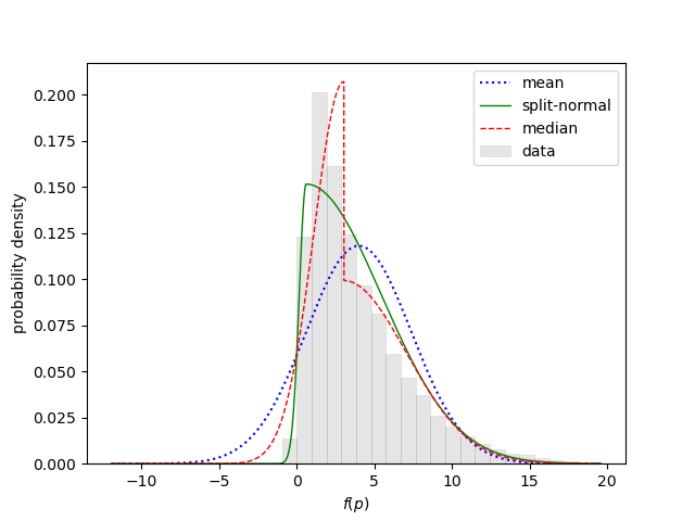
shows the statistical analysis for fp:

Statistics for fp:
   mean = 3.9920(59)   sdev = 3.369(15)   skew = 1.655(23)   ex_kurt = 3.99(16)
   split-normal: 0.5988(22) +/- 4.839(12)/0.4289(47)
         median: 3.0411(66) +/- 4.009(17)/1.9274(76)

g_ev.stats(f, moments=True, histograms=True) calculates moments for each output quantity, and uses the moments to determines the mean, standard deviation, skewness, and excess kurtosis of each distribution. It also calculates a histogram for each distribution and fits the histogram with two two-sided Gaussian models: one that is continuous (split-normal), and the other that is discontinuous centered on the median. The uncertainties shown for each quantity come from the vegas integrations.

The last line in the code above displays the histogram for fp, which confirms that it is not particularly Gaussian:

The discussion in Case Study: Bayesian Curve Fitting illustrates how vegas.PDFIntegrator can be used with a non-Gaussian PDF in two examples, one with 4 parameters and the other with 22 parameters. It also shows how to use vegas.PDFIntegrator.sample() to create (weighted) random samples of parameter points whose density is proportional to the integrator’s PDF.

Finally, note that the lsqfit Python module uses vegas.PDFIntegrator to implement a least-squares fitter vegas_fit that uses Bayesian integration (rather than minimization).

Faster Integrands¶

The computational cost of a realistic multidimensional integral comes mostly from the cost of evaluating the integrand at the Monte Carlo sample points. Integrands written in pure Python are probably fast enough for problems where neval=1e3 or neval=1e4 gives enough precision. Some problems, however, require hundreds of thousands or millions of function evaluations, or more.

We can significantly reduce the cost of evaluating the integrand by using vegas’s batch mode. For example, replacing

import vegas
import math

def f(x):
    dim = len(x)
    norm = 1013.2118364296088 ** (dim / 4.)
    dx2 = 0.0
    for d in range(dim):
        dx2 += (x[d] - 0.5) ** 2
    return math.exp(-100. * dx2) * norm

integ = vegas.Integrator(4 * [[0, 1]])

integ(f, nitn=10, neval=2e5)
result = integ(f, nitn=10, neval=2e5)
print('result = %s   Q = %.2f' % (result, result.Q))

by

import vegas
import numpy as np

@vegas.llbatchintegrand
def f_batch(x):
    # evaluate integrand at multiple points simultaneously
    dim = x.shape[1]
    norm = 1013.2118364296088 ** (dim / 4.)
    dx2 = 0.0
    for d in range(dim):
        dx2 += (x[:, d] - 0.5) ** 2
    return np.exp(-100. * dx2) * norm

integ = vegas.Integrator(4 * [[0, 1]])

integ(f_batch, nitn=10, neval=2e5)
result = integ(f_batch, nitn=10, neval=2e5)
print('result = %s   Q = %.2f' % (result, result.Q))

reduces the cost of the integral by an order of magnitude. Internally vegas processes integration points in batches. (vegas parameter min_neval_batch determines the number of integration points per batch (typically 10,000s).) In batch mode, vegas presents integration points to the integrand in batches rather than offering them one at a time. Here, for example, function f_batch(x) accepts an array of integration points — x[i, d] where i=0... labels the integration point and d=0... the direction — and returns an array of integrand values corresponding to those points. The decorator vegas.lbatchintegrand() tells vegas that it should send integration points to f(x) in batches.

An alternative to a function decorated with vegas.lbatchintegrand() is a class that behaves like a batch integrand:

import vegas
import numpy as np

@vegas.lbatchintegrand
class f_batch:
    def __init__(self, dim):
        self.dim = dim
        self.norm = 1013.2118364296088 ** (dim / 4.)

    def __call__(self, x):
        # evaluate integrand at multiple points simultaneously
        dx2 = 0.0
        for d in range(self.dim):
            dx2 += (x[:, d] - 0.5) ** 2
        return np.exp(-100. * dx2) * self.norm

f = f_batch(dim=4)
integ = vegas.Integrator(f.dim * [[0, 1]])

integ(f, nitn=10, neval=2e5)
result = integ(f, nitn=10, neval=2e5)
print('result = %s   Q = %.2f' % (result, result.Q))

This version is as fast as the previous batch integrand, but is potentially more flexible because it is built around a class rather than a function. (Some classes won’t allow decorators. An alternative to the decorator is to derive the class from vegas.LBatchIntegrand.)

The batch integrands here are fast because they are expressed in terms numpy operators that act on entire arrays — they evaluate the integrand for all integration points in a batch at the same time. That optimization is not always possible or simple. It is unnecessary if we write the integrand in Cython, which is a compiled hybrid of Python and C. The Cython version of the (batch) integrand is:

# file: cython_integrand.pyx

import numpy as np

# use exp from C
from libc.math cimport exp

def f_batch(double[:, ::1] x):
    cdef int i          # labels integration point
    cdef int d          # labels direction
    cdef int dim = x.shape[1]
    cdef double norm = 1013.2118364296088 ** (dim / 4.)
    cdef double dx2
    cdef double[::1] ans = np.empty(x.shape[0], float)
    for i in range(x.shape[0]):
        # integrand for integration point x[i]
        dx2 = 0.0
        for d in range(dim):
            dx2 += (x[i, d] - 0.5) ** 2
        ans[i] = exp(-100. * dx2) * norm
    return ans

We put this in a separate file called, say, cython_integrand.pyx, and rewrite the main code as:

import numpy as np
import pyximport
pyximport.install(inplace=True)

import vegas
from cython_integrand import f_batch
f = vegas.lbatchintegrand(f_batch)

integ = vegas.Integrator(4 * [[0, 1]])

integ(f, nitn=10, neval=2e5)
result = integ(f, nitn=10, neval=2e5)
print('result = %s   Q = %.2f' % (result, result.Q))

Module pyximport is used here to cause the Cython module cython_integrand.pyx to be compiled the first time it is imported. The compiled code is used in subsequent imports, so compilation occurs only once.

Batch mode is also useful for array-valued integrands. The code from the previous section could have been written as:

import vegas
import gvar as gv
import numpy as np

dim = 4

@vegas.lbatchintegrand
def f(x):
    ans = np.empty((x.shape[0], 3), float)
    dx2 = 0.0
    for d in range(dim):
        dx2 += (x[:, d] - 0.5) ** 2
    ans[:, 0] = np.exp(-200 * dx2)
    ans[:, 1] = x[:, 0] * ans[:, 0]
    ans[:, 2] = x[:, 0] ** 2 * ans[:, 0]
    return ans

integ = vegas.Integrator(4 * [[0, 1]])

# adapt grid
training = integ(f, nitn=10, neval=2000)

# final analysis
result = integ(f, nitn=10, neval=10000)
print('I[0] =', result[0], '  I[1] =', result[1], '  I[2] =', result[2])
print('Q = %.2f\n' % result.Q)
print('<x> =', result[1] / result[0])
print(
    'sigma_x**2 = <x**2> - <x>**2 =',
    result[2] / result[0] - (result[1] / result[0]) ** 2
    )
print('\ncorrelation matrix:\n', gv.evalcorr(result))

Note that the batch index (here :) always comes first. An extra (first) index is also added to each value in the dictionary returned by a dictionary-valued batch integrand: e.g.,

dim = 4

@vegas.lbatchintegrand
def f(x):
    ans = {}
    dx2 = 0.0
    for d in range(dim):
        dx2 += (x[:, d] - 0.5) ** 2
    ans['1'] = np.exp(-200 * dx2)
    ans['x'] = x[:, 0] * ans['1']
    ans['x**2'] = x[:, 0] ** 2 * ans['1']
    return ans

It is sometimes more convenient to have the batch index be the last index (the rightmost) rather than the first. Then @vegas.lbatchintegrand is replaced by @vegas.rbatchintegrand, and vegas.LBatchIntegrand by vegas.RBatchIntegrand. (Note that @vegas.batchintegrand and @vegas.lbatchintegrand are the same, as are vegas.BatchIntegrand and vegas.LBatchIntegrand.)

Multiple Processors¶

vegas supports parallel evaluation of integrands on multiple processors. This can shorten execution time substantially when the integrand is costly to evaluate. The following code, for example, runs more than five times faster when using nproc=8 processors instead of the default nproc=1 (on a 2019 laptop):

import vegas
import numpy as np

# Integrand: ridge of N Gaussians spread along part of the diagonal
def ridge(x):
    N = 10000
    x0 = np.linspace(0.4, 0.6, N)
    dx2 = 0.0
    for xd in x:
        dx2 += (xd - x0) ** 2
    return np.average(np.exp(-100. * dx2)) *  (100. / np.pi) ** (len(x) / 2.)

def main():
    integ = vegas.Integrator(4 * [[0, 1]], nproc=8)  # 8 processors
    # adapt
    integ(ridge, nitn=10, neval=1e4)
    # final results
    result = integ(ridge, nitn=10, neval=1e4)
    print('result = %s    Q = %.2f' % (result, result.Q))

if __name__ == '__main__':
    main()

The code doesn’t run eight times faster because it takes time to initiate the nproc processes, and to feed data and collect results from them. Parallel processing only becomes useful when integrands are sufficiently costly that such overheads become negligible.

Parallel processing is managed by Python’s multiprocessing module. The if __name__ == '__main__' construct at the end of this code is essential when running on Windows or MacOS (in its default mode) as it prevents additional processes being launched when the main module is imported as part of spawning the nproc processes; see the multiprocessing documentation for more details. This is not an issue for Linux/Unix. It is also important that the integrand and its return values can be pickled using Python’s pickle module. This is the case for most pure Python integrands.

The code above will generate an AttributeError when run in some interactive environments (as opposed to running from the command line) on some platforms. This can usually be fixed by putting the integrand function ridge(x) into a file and importing it into the script.

vegas also supports multi-processor evaluation of integrands using MPI (via the Python module mpi4py which must be installed separately). Placing the code above in a file ridge.py, with mpi=True set in the integrator (and with nproc=1 or unset) —

integ = vegas.Integrator(4 * [[0, 1]], mpi=True)

— ridge.py can be run on 8 processors using

mpirun -np 8 python ridge.py

The speedup is similar to that from using the multiprocessing module, above. Note that the random number generator used by vegas must be synchronized so that it produces the same random numbers on the different processors. This happens automatically for the default random-number generator.

vegas’s batch mode makes it possible to implement other strategies for distributing integrand evaluations across multiple processors. For example, we can create a class parallelintegrand whose function is similar to decorator vegas.batchintegrand(), but where Python’s multiprocessing module provides parallel processing:

import multiprocessing
import numpy as np
import vegas

class parallelintegrand(vegas.BatchIntegrand):
    """ Convert (batch) integrand into multiprocessor integrand.

    Integrand should return a numpy array.
    """
    def __init__(self, fcn, nproc=4):
        " Save integrand; create pool of nproc processes. "
        super().__init__()
        self.fcn = fcn
        self.nproc = nproc
        self.pool = multiprocessing.Pool(processes=nproc)
    def __del__(self):
        " Standard cleanup. "
        self.pool.close()
        self.pool.join()
    def __call__(self, x):
        " Divide x into self.nproc chunks, feeding one to each process. "
        nx = x.shape[0] // self.nproc + 1
        # launch evaluation of self.fcn for each chunk, in parallel
        results = self.pool.map(
            self.fcn,
            [x[i*nx : (i+1)*nx] for i in range(self.nproc)],
            1,
            )
        # convert list of results into a single numpy array
        return np.concatenate(results)

Then fparallel = parallelintegrand(f, 4), for example, will create a new integrand fparallel(x) that uses 4 CPU cores.

Sums with `vegas`¶

The code in the previous sections is inefficient in the way it handles the sum over 10,000 Gaussians. It is not necessary to include every term in the sum for every integration point. Rather we can sample the sum, using vegas to do the sampling. The trick is to replace the sum with an equivalent integral:

$\frac{1}{N}\sum_{i=0}^{N-1} f(i) = \int_0^1 dx \; f(\mathrm{floor}(x N))$

where $\mathrm{floor}(x)$ is the largest integer smaller than $x$ . The resulting integral can then be handed to vegas. Using this trick, the integral in the previous section can be re-cast as a 5-dimensional integral:

import vegas
import numpy as np

# Integrand: ridge of N Gaussians spread evenly along the diagonal
def ridge(x):
    N = 10000
    dim = 4
    x0 = 0.4 + 0.2 * np.floor(x[-1] * N) / (N - 1.)
    dx2 = 0.0
    for xd in x[:-1]:
        dx2 += (xd - x0) ** 2
    return np.exp(-100. * dx2) *  (100. / np.pi) ** (dim / 2.)

def main():
    integ = vegas.Integrator(5 * [[0, 1]])
    # adapt
    integ(ridge, nitn=10, neval=5e4)
    # final results
    result = integ(ridge, nitn=10, neval=5e4)
    print('result = %s    Q = %.2f' % (result, result.Q))

if __name__ == '__main__':
    main()

This code gives a result with the same precision, but is 5x faster than the code in the previous section (with nproc=1; it is another 3x faster when nproc=8).

The same trick can be generalized to sums over multiple indices, including sums to infinity. vegas will provide Monte Carlo estimates of the sums, emphasizing the more important terms.

Saving Results Automatically¶

Results returned by a vegas integrator can be pickled for later use using pickle.dump/load (or gvar.dump/load) in the usual way. Results can also be saved automatically using the save keyword to specify a file name for the pickled result: for example, running

import vegas
import math

def f(x):
    dx2 = 0
    for d in range(4):
        dx2 += (x[d] - 0.5) ** 2
    return math.exp(-dx2 * 100.) * 1013.2118364296088

integ = vegas.Integrator([[-2, 2], [0, 2], [0, 2], [0, 2]])

result = integ(f, nitn=10, neval=1000, save='save.pkl')
print(result.summary())
print('result = %s    Q = %.2f' % (result, result.Q))

prints out

itn   integral        wgt average     chi2/dof        Q
-------------------------------------------------------
 0.00050(45)     0.00050(45)         0.00     1.00
 0.115(59)       0.00051(45)         3.77     0.05
 0.66(22)        0.00051(45)         6.41     0.00
 0.72(15)        0.00052(45)        12.27     0.00
 0.97(12)        0.00053(45)        26.17     0.00
 1.045(61)       0.00059(45)        79.46     0.00
 1.016(45)       0.00069(45)       152.45     0.00
 1.023(29)       0.00093(45)       307.32     0.00
 0.999(20)       0.00141(45)       573.82     0.00
 1.025(17)       0.00208(45)       896.20     0.00

result = 0.00208(45)    Q = 0.00

but also stores result in file save.pkl. The result can be retrieved later using, for example,

import pickle

with open('save.pkl', 'rb') as ifile:
    result = pickle.load(ifile)

print(result.summary())
print('result = %s    Q = %.2f' % (result, result.Q))

which gives exactly the same output.

This feature is most useful for expensive integrations, ones taking minutes or hours to complete. This is because the pickled file is updated after every vegas iteration. This means that a short script like the one above can be used to monitor progress before the integration is finished. It also means that results up through the most recent iteration are saved even if the integration is terminated early or crashes.

Saved results are also useful because they can be fixed after the code has finished running. The early iterations in the output above are clearly wrong and badly distort the weighted average. The problem is that vegas isn’t well adapted to the integrand until around the fifth or sixth iteration. We can discard the first five iterations (from the saved result) by using function vegas.ravg() to redo the weighted average:

import pickle
import vegas

with open('save.pkl', 'rb') as ifile:
    result = pickle.load(ifile)
result = vegas.ravg(result.itn_results[5:])

print(result.summary())
print('result = %s    Q = %.2f' % (result, result.Q))

This gives the following output

itn   integral        wgt average     chi2/dof        Q
-------------------------------------------------------
  1   1.045(61)       1.045(61)           0.00     1.00
  2   1.016(45)       1.026(36)           0.14     0.71
  3   1.023(29)       1.024(23)           0.07     0.93
  4   0.999(20)       1.010(15)           0.28     0.84
  5   1.025(17)       1.017(11)           0.31     0.87

result = 1.017(11)    Q = 0.87

which is greatly improved over the original.

It is also possible to save an adapted integrator using pickle.dump/load (or gvar.dump/load). This can also be done automatically, by replacing, for example, save='save.pkl' with saveall='saveall.pkl' in the script above. The pickled file then returns a tuple containing the most recent result and integ. Having the (adapted) integrator, it is possible to further refine a result later: for example, running

import pickle

def f(x):
    dx2 = 0
    for d in range(4):
        dx2 += (x[d] - 0.5) ** 2
    return math.exp(-dx2 * 100.) * 1013.2118364296088

with open('saveall.pkl', 'rb') as ifile:
    result, integ = pickle.load(ifile)
result = vegas.ravg(result.itn_results[5:])

new_result = integ(f, nitn=5)

print('\nNew results:')
print(new_result.summary())

print('\nCombined results:')
result.extend(new_result)
print(result.summary())
print('Combined result = %s    Q = %.2f' % (result, result.Q))

significantly improves the final result by adding 5 additional iterations to what was done earlier. The new iterations are in new_result and tabulated under “New Results” in the output:

New results:
itn   integral        wgt average     chi2/dof        Q
-------------------------------------------------------
  1   1.007(17)       1.007(17)           0.00     1.00
  2   1.006(14)       1.007(11)           0.00     0.98
  3   0.997(13)       1.0029(82)          0.16     0.85
  4   1.015(21)       1.0044(76)          0.20     0.90
  5   0.990(13)       1.0007(66)          0.39     0.82


Combined results:
itn   integral        wgt average     chi2/dof        Q
-------------------------------------------------------
  1   1.045(61)       1.045(61)           0.00     1.00
  2   1.016(45)       1.026(36)           0.14     0.71
  3   1.023(29)       1.024(23)           0.07     0.93
  4   0.999(20)       1.010(15)           0.28     0.84
  5   1.025(17)       1.017(11)           0.31     0.87
  6   1.007(17)       1.0136(94)          0.30     0.91
  7   1.006(14)       1.0114(78)          0.28     0.95
  8   0.997(13)       1.0076(66)          0.36     0.92
  9   1.015(21)       1.0082(63)          0.33     0.95
 10   0.990(13)       1.0047(57)          0.48     0.89

Combined result = 1.0047(57)    Q = 0.89

The new results are merged onto the end of the original results using result.extend(new_result) to obtain the combined results from all 10 iterations (old plus new).

Saving integrators is again useful for costly integrations that might need to be restarted later since the saved integrator remembers the variable transformations made to minimize errors, and so need not be readapted to the integrand when used again. The resulting pickle file can be large, however, particularly if neval is large. The (adapted) vegas.AdaptiveMap integ.map can also be pickled by itself and results in a smaller file.

`vegas` Maps and Preconditioning `vegas`¶

vegas adapts by remapping the integration variables (see Importance Sampling). It is possible to precondition this map, before creating a vegas.Integrator. Preconditioned maps can improve vegas results when much is known about the integrand ahead of time. Consider, for example, the integral

$C\int_0^1 \!d^5x\, \,\sum_{i=1}^2 \mathrm{e}^{-50 |\mathbf{x} - \mathbf{r}_i|},$

which has high, narrow peaks at

$\mathbf{r}_1 = (0.45, 0.45, 0.45, 0.45, 0.45),$

$\mathbf{r}_2 = (0.7, 0.7, 0.7, 0.7, 0.7).$

Given the locations of the peaks we can create a vegas map before integrating that emphasizes the regions around them:

import vegas
import numpy as np

@vegas.batchintegrand
def f(x):
    ans = 0
    for c in [0.45, 0.7]:
        dx2 = np.sum((x - c) ** 2, axis=1)
        ans += np.exp(-50 * np.sqrt(dx2))
    return ans * 247366.171

dim = 5
map = vegas.AdaptiveMap(dim * [[0, 1]])     # uniform map
x = np.concatenate([                        # 2000 points near peaks
    np.random.normal(loc=0.45, scale=3/50, size=(1000, dim)),
    np.random.normal(loc=0.7, scale=3/50, size=(1000, dim)),
    ])
map.adapt_to_samples(x, f(x), nitn=5)       # precondition map
integ = vegas.Integrator(map, alpha=0.)
r = integ(f, neval=1e4, nitn=5)
print(r.summary())

vegas maps are objects of type vegas.AdaptiveMap. Here we create a uniform map object map. We then generate 2000 random points x from normal distributions centered around the peak locations. map.adapt_to_samples(x, f(x), nitn=5) optimizes the map for integrating f(x) based on information about the integrand at the random points x. As a result, vegas is almost fully adapted to the integrand already in its first iteration:

itn   integral        wgt average     chi2/dof        Q
-------------------------------------------------------
 0.981(25)       0.981(25)           0.00     1.00
 0.983(11)       0.9825(98)          0.00     0.96
 1.001(10)       0.9915(71)          0.85     0.43
 1.000(13)       0.9933(63)          0.67     0.57
 0.993(11)       0.9931(54)          0.50     0.74

We set alpha=0 in the integrator to prevent further changes to the pre-adapted map.

These results can be contrasted with what happens without preconditioning, where the integrator is still far from converged by the fifth iteration:

itn   integral        wgt average     chi2/dof        Q
-------------------------------------------------------
 0.74(27)        0.74(27)            0.00     1.00
 0.93(12)        0.90(11)            0.38     0.54
 0.94(10)        0.920(74)           0.23     0.79
 1.091(75)       1.004(53)           1.03     0.38
 1.063(58)       1.031(39)           0.91     0.46

The exact distribution of random points x isn’t important; what matters is that they cover and are concentrated in the dominant regions contributing to the integral. Should it be needed, a sample xsample=(x, f(x)) in x-space is easily converted to the equivalent sample in y-space using:

x, fx = xsample
y = np.empty(x.shape, float)
jac = np.empty(x.shape[0], float)
map.invmap(x, y, jac)
ysample = (y, jac * fx)

where map.invmap(x, y, jac) fills array y with the y-space points corresponding to x, and array jac with the transformation’s Jacobian.

Note that vegas maps can be used with integrators other than vegas. The vegas map maps the integration variables x[d] into new variables y[d] (where 0 < y[d] < 1) that make the integrand easier to integrate. The integrator is used to evaluate the integral in y-space. To illustrate how this works, we replace the last three lines of the code at the start of this section with the following:

def smc(f, neval, dim):
    " integrates f(y) over dim-dimensional unit hypercube "
    y = np.random.uniform(0,1, (neval, dim))
    fy = f(y)
    return (np.average(fy), np.std(fy) / neval ** 0.5)

def g(y):
    jac = np.empty(y.shape[0], float)
    x = np.empty(y.shape, float)
    map.map(y, x, jac)
    return jac * f(x)

# with map
r = smc(g, 50_000, dim)
print('   SMC + map:', f'{r[0]:.3f} +- {r[1]:.3f}')

# without map
r = smc(f, 50_000, dim)
print('SMC (no map):', f'{r[0]:.3f} +- {r[1]:.3f}')

Here smc is a Simple Monte Carlo (SMC) integrator and g(y) is the integrand in y-space that corresponds to f(x) in x-space. The mapping is done by map.map(y, x, jac) which fills the arrays x and jac with the x values and Jacobian corresponding to integration points y. The result is

   SMC + map: 1.013 +- 0.020
SMC (no map): 1.703 +- 0.535

where we give results from SMC with and without using the vegas map. The vegas map greatly improves the SMC result, which, not surprisingly, is significantly less accurate the the vegas result above. Maps for use with other integrators can be built directly, as above, or they can be built for a particular integrand by running several iterations of vegas with the integrand and using the vegas integrator’s map: integ.map.

`vegas` Stratifications¶

Having mapped the integration variables x[d] to new variables y[d], vegas evaluates the integral in y-space using stratified Monte Carlo sampling (see Adaptive Stratified Sampling). This is done by dividing each axis d into nstrat[d] equal stratifications, which divide the D-dimensional integration volume into prod(nstrat) sub-volumes or (rectangular) hypercubes. vegas does a separate integral in each hypercube, adjusting the number of integrand evaluations used in each one to minimize errors. By default, the number of stratifications is set automatically based on the number neval of integrand evaluations per iteration: nstrat[d] is set equal to $M_\mathrm{st}+1$ for the first $D_0$ directions and $M_\mathrm{st}$ for the remaining directions, where $M_\mathrm{st}$ and $D_0$ are chosen to maximize the number stratifications consistent with neval. It is also possible, however, to specify the number of stratifications nstrat[d] for each direction separately.

Requiring (approximately) the same number of stratifications in each direction greatly limits the number of stratifications in very high dimensions, since the product of the nstrat[d] must be less than neval/2 (so there are at least two integrand samples in each hypercube). This restricts vegas’s ability to adapt. Often there is a subset of integration directions that are more challenging than the others. In high dimensions (and possibly lower dimensions) it is worthwhile using larger values for nstrat[d] for those directions.

An example is the 20-dimensional integral

$C\int_0^1 \!d^{20}x\, \,\sum_{i=1}^3 \mathrm{e}^{-100 (\mathbf{x} - \mathbf{r}_i)^2},$

which has high, narrow peaks at

$\mathbf{r}_1 = (0.23, 0.23, 0.23, 0.23, 0.23, 0.45, \ldots, 0.45),$

$\mathbf{r}_2 = (0.39, 0.39, 0.39, 0.39, 0.39, 0.45, \ldots, 0.45),$

$\mathbf{r}_3 = (0.74, 0.74, 0.74, 0.74, 0.74, 0.45, \ldots, 0.45).$

These peaks are aligned along the diagonal of the integration volume for the first five directions, but are on top of each other in the remaining directions. This makes the integrals over the first five directions much more challenging than the remaining integrals.

To integrate this function, we specify nstrat[d] rather than neval. We set nstrat[d]=10 for the first five directions, and nstrat[d]=1 for all the rest. This fixes the number of function evaluations to be approximately eight times the number of hypercubes created by the stratifications (i.e., eight times 100,000), which provides enough integrand samples for adaptive stratified sampling while also guaranteeing at least two samples per hypercube. The following code

import vegas
import numpy as np

dim = 20
r = np.array([
    5 * [0.23] + (dim - 5) * [0.45],
    5 * [0.39] + (dim - 5) * [0.45],
    5 * [0.74] + (dim - 5) * [0.45],
    ])

@vegas.batchintegrand
def f(x):
    ans = 0
    for ri in r:
        dx2 = np.sum((x - ri[None, :]) ** 2, axis=1)
        ans += np.exp(-100 * dx2)
    return ans * 356047712484621.56

integ = vegas.Integrator(dim * [[0, 1]], alpha=0.25)
nstrat = 5 * [10] + (dim - 5) * [1]
integ(f, nitn=15, nstrat=nstrat)            # warmup
r = integ(f, nitn=5, nstrat=nstrat)
print(r.summary())
print('nstrat =', np.array(integ.nstrat))

gives excellent results:

itn   integral        wgt average     chi2/dof        Q
-------------------------------------------------------
  1   0.920(50)       0.920(50)           0.00     1.00
  2   0.993(30)       0.974(26)           1.60     0.21
  3   1.014(30)       0.990(20)           1.30     0.27
  4   1.099(64)       0.999(19)           1.73     0.16
  5   1.0028(78)      1.0023(72)          1.31     0.26

nstrat = [10 10 10 10 10  1  1  1  1  1  1  1  1  1  1  1  1  1  1  1]

vegas struggles to converge, however, when in its default mode with the same number of integrand evaluations (about 800,000 per iteration):

itn   integral        wgt average     chi2/dof        Q
-------------------------------------------------------
  1   2.1(1.4)        2.1(1.4)            0.00     1.00
  2   0.637(42)       0.638(42)           1.14     0.29
  3   0.755(53)       0.684(33)           2.06     0.13
  4   0.750(49)       0.704(27)           1.78     0.15
  5   0.89(11)        0.716(27)           2.07     0.08

nstrat = [2 2 2 2 2 2 2 2 2 2 2 2 2 2 2 2 1 1 1 1]

`vegas` Jacobian¶

The vegas Jacobian is useful when integrating multiple integrands simultaneously when some of the integrands depend only on a subset of the integration variables.

Consider, for example, the integral

$\int^{\pi/2}_0 dx_0 \, \frac{1}{(x_0-\delta)^2 + 0.01}.$

We want to compare this integral for two different cases: a) where $\delta=x_1$ is a random number near zero drawn from a distribution proportional to $\mathrm{exp}(-100\, \mathrm{sin} (x_1))$ with $0\le x_1 \le \pi/2$ ; and b) where $\delta=0$ . The result for the first case is $I_a = I_a^\mathrm{num}/I_a^\mathrm{den}$ where

$I_a^\mathrm{num} &= \int^{\pi/2}_0 dx_0 \int^{\pi/2}_0 dx_1 \, \mathrm{e}^{-100\,\mathrm{sin}(x_1)} \, \frac{1}{(x_0-x_1)^2 + 0.01} \\ I_a^\mathrm{den} &= \int^{\pi/2}_0 dx_1 \, \mathrm{e}^{-100 \,\mathrm{sin}(x_1)}.$

The result for the second case is

$I_b = \int^{\pi/2}_0 dx_0 \, \frac{1}{(x_0)^2 + 0.01}.$

The first two integrals should have very similar dependence on $x_1$ , while the first and third integrals should have similar dependence on $x_0$ . Given these similarities, we would like to do all three integrals simultaneously; but one integral is two-dimensional and the other two are one-dimensional.

One solution is to turn the one-dimensional integrals into two-dimensional integrals by rewriting $I_a^\mathrm{den}$ as

$I_a^\mathrm{den} &= \int^{\pi/2}_0 \frac{dx_0}{\pi/2} \int^{\pi/2}_0 dx_1 \, \mathrm{e}^{-100 \,\mathrm{sin}(x_1)}.$

and similarly for $I_b$ . These are then easily integrated together —

import vegas
import numpy as np

integ = vegas.Integrator(2 * [(0., np.pi/2.)])

@vegas.rbatchintegrand
def f(x):
    Ia_num = np.exp(-1e2 * np.sin(x[1])) / ((x[0] - x[1])**2 + 0.01)
    Ia_den = np.exp(-1e2 * np.sin(x[1])) / (np.pi/2)
    Ib = 1 /  (x[0]**2 + 0.01) / (np.pi/2)
    return dict(Ia_num=Ia_num, Ia_den=Ia_den, Ib=Ib)

w = integ(f, neval=20000, nitn=10)
r = integ(f, neval=20000, nitn=5)
print(r.summary(True))
print('Ia =', r['Ia_num'] / r['Ia_den'], 'Ia - Ib =', r['Ia_num'] / r['Ia_den'] - r['Ib'])

— but the result is useless:

itn   integral        wgt average     chi2/dof        Q
-------------------------------------------------------
  1   0.160568(44)    0.160568(44)        0.00     1.00
  2   0.160551(40)    0.160559(30)        0.13     0.94
  3   0.160533(35)    0.160549(23)        0.36     0.90
  4   0.160568(32)    0.160555(18)        0.96     0.47
  5   0.160553(29)    0.160554(15)        0.73     0.72

  key/index             value
-----------------------------
     Ia_num     0.160554 (15)
     Ia_den    0.0099995 (60)
         Ib        14.62 (88)

Ia = 16.0562(99) Ia - Ib = 1.43(88)

$I_b$ is almost 100x less accurate than $I_a$ , despite having an integrand with no x[1] dependence. The problem is that the vegas map for x[1] is tailored to $I_a^\mathrm{num}$ , which has a strong peak at x[1]=0. That map is highly sub-optimal for integrating a function, like that in $I_b$ , that is independent of x[1].

A much better approach is to rewrite the one-dimensional integrals as two-dimensional integrals using the vegas map’s Jacobian $dx_d/dy_d$ in the extra direction $d$ . For example,

$I_a^\mathrm{den} &= \int^{\pi/2}_0 \frac{dx_0}{dx_0/dy_0} \int^{\pi/2}_0 dx_1 \, \mathrm{e}^{-100 \,\mathrm{sin}(x_1)}.$

This turns the $x_0$ integral into an integral over $0\le y_0 \le 1`$ with an integrand equal to 1. The Monte Carlo integral over $y_0$ in vegas is then exact; it is unaffected by the map for that direction. This is easily implemented for both one-dimensional integrals by setting keyword uses_jac=True in the integrator and modifying the integrand:

@vegas.rbatchintegrand
def f(x, jac):
    Ia_num = np.exp(-1e2 * np.sin(x[1])) / ((x[0] - x[1])**2 + 0.01)
    Ia_den = np.exp(-1e2 * np.sin(x[1])) / jac[0]
    Ib = 1 /  (x[0]**2 + 0.01) / jac[1]
    return dict(Ia_num=Ia_num, Ia_den=Ia_den, Ib=Ib)

w = integ(f, uses_jac=True, neval=20000, nitn=10)
r = integ(f, uses_jac=True, neval=20000, nitn=5)

Setting uses_jac=True causes vegas to call the integrand with two arguments instead of one: f(x, jac=jac) where jac[d] is the Jacobian for direction d (array jac has the same shape as x). This gives much better results —

itn   integral        wgt average     chi2/dof        Q
-------------------------------------------------------
  1   0.160568(44)    0.160568(44)        0.00     1.00
  2   0.160551(40)    0.160560(30)        0.28     0.84
  3   0.160533(35)    0.160547(22)        0.38     0.89
  4   0.160568(32)    0.160554(18)        0.58     0.82
  5   0.160553(29)    0.160553(15)        0.58     0.86

  key/index              value
------------------------------
     Ia_num      0.160553 (15)
     Ia_den    0.01000103 (59)
         Ib       15.0749 (11)

Ia = 16.0536(12) Ia - Ib = 0.97868(38)

— where now $I_a$ and $I_b$ are comparable in precision and the difference is quite accurate. Note that the error on the difference is smaller than either of the separate errors, because of correlations between the two results.

`vegas` as a Random Number Generator¶

A vegas integrator generates random points in its integration volume from a distribution that is optimized for integrals of whatever function it was trained on. The integrator provides low-level access to the random-point generator through the iterators vegas.Integrator.random() and vegas.Integrator.random_batch().

To illustrate, the following code snippet estimates the integral of function f(x) using integrator integ:

integral = 0.0
for x, wgt in integ.random():
    integral += wgt * f(x)

Here x[d] is a random point in the integration volume and wgt is the weight vegas assigns to that point in an integration. The iterator generates integration points and weights corresponding to a single iteration of the vegas algorithm. In practice, we would train integ on a function whose shape is similar to that of f(x) before using it to estimate the integral of f(x).

It is usually more efficient to generate and use integration points in batches. The vegas.Integrator.random_batch() iterator does just this:

integral = 0.0
for x, wgt in integ.random_batch():
    integral += wgt.dot(batch_f(x))

Here x[i, d] is an array of integration points, wgt[i] contains the corresponding weights, and batch_f(x) returns an array containing the corresponding integrand values.

The random points generated by vegas are stratified into hypercubes: vegas uses transformed integration variables to improve its Monte Carlo estimates. It further improves those estimates by subdividing the integration volume in the transformed variables into a large number of hypercubes, and doing a Monte Carlo integral in each hypercube separately (see previous section). The final result is the sum of the results from all the hypercubes.

To mimic a full vegas integral estimate using the iterators above, we need to know which points belong to which hypercubes. The following code shows how this is done:

import gvar as gv

integral = 0.0
variance = 0.0
for x, wgt, hcube in integ.random_batch(yield_hcube=True):
    wgt_fx = wgt * batch_f(x)
    # iterate over hypercubes: compute variance for each,
    #                          and accumulate for final result
    for i in range(hcube[0], hcube[-1] + 1):
        idx = (hcube == i)          # select array items for h-cube i
        nwf = np.sum(idx)           # number of points in h-cube i
        wf = wgt_fx[idx]
        sum_wf = np.sum(wf)         # sum of wgt * f(x) for h-cube i
        sum_wf2 = np.sum(wf ** 2)   # sum of (wgt * f(x)) ** 2
        integral += sum_wf
        variance += (sum_wf2 * nwf - sum_wf ** 2) / (nwf - 1.)
# answer = integral;   standard deviation = variance ** 0.5
result = gv.gvar(integral, variance ** 0.5)

Here hcube[i] identifies the hypercube containing x[i, d]. This example is easily modified to provide information about the vegas Jacobian to the integrand, if needed (see the section vegas Jacobian):

integral = 0.0
variance = 0.0
for x, y, wgt, hcube in integ.random_batch(yield_hcube=True, yield_y=True):
    wgt_fx = wgt * batch_f(x, jac=integ.map.jac1d(y))
    ...

The example is also easily modified for integrands batch_f(xd) where xd is a dictionary:

integral = 0.0
variance = 0.0
for x, wgt, hcube in integ.random_batch(yield_hcube=True):
    xd = gv.BufferDict(integ.xdict, lbatch_buf=x)
    wgt_fx = wgt * batch_f(xd)
    ...

Here integ.xdict provides the template dictionary used to construct the dictionary xd.

Implementation Notes¶

This implementation relies upon Cython for its speed and numpy for array processing. It also uses matplotlib for graphics, h5py when minimize_mem=True, and mpi4py for MPI support, but these are all optional.

vegas also uses the gvar module (pip install gvar). Integration results are returned as objects of type gvar.GVar, which is a class representing Gaussian random variables (i.e., something with a mean and standard deviation). These objects can be combined with numbers and with each other in arbitrary arithmetic expressions to get new gvar.GVars with the correct standard deviations, and properly correlated with other gvar.GVars — that is the tricky part.

Tutorial¶

Introduction¶

Basic Integrals¶

Multiple Integrands Simultaneously¶

Dictionaries¶

Calculating Distributions¶

PDF Integrals¶

Faster Integrands¶

Multiple Processors¶

Sums with `vegas`¶

Saving Results Automatically¶

`vegas` Maps and Preconditioning `vegas`¶

`vegas` Stratifications¶

`vegas` Jacobian¶

`vegas` as a Random Number Generator¶

Implementation Notes¶

Table of Contents

Previous topic

Next topic

This Page

Tutorial¶

Introduction¶

Basic Integrals¶

Multiple Integrands Simultaneously¶

Dictionaries¶

Calculating Distributions¶

PDF Integrals¶

Faster Integrands¶

Multiple Processors¶

Sums with vegas¶

Saving Results Automatically¶

vegas Maps and Preconditioning vegas¶

vegas Stratifications¶

vegas Jacobian¶

vegas as a Random Number Generator¶

Implementation Notes¶

Sums with `vegas`¶

`vegas` Maps and Preconditioning `vegas`¶

`vegas` Stratifications¶

`vegas` Jacobian¶

`vegas` as a Random Number Generator¶